1. Xavier Weight Initialization
Xavier Glorot and Yoshua Bengio (2010) considered random initialized networks and the associated variance of pre-activation values and the gradients as they pass from layer to layer. Glorot and Bengio noted that for symmetric \(\phi(\cdot)\) such as \(\tanh(\cdot)\), the hidden layer values are approximately Gaussian with a variance depending on the variance of the weight matrices \(W^{(i)}\).
In particular, if \(\sigma_W\) is selected appropriately (\(\sigma_W^2=1/(3n)\)) then the variance of hidden layer values is approximately constant through layers (bottom plot of Figure 1); if \(\sigma_W\) is small then the variance of hidden layer values converges towards zero with depth (top plot of Figure 1).
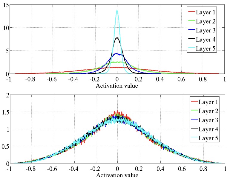
Similarly, the gradient of a loss function used for training shows the similar Gaussian behavior depending on \(\sigma_W\).
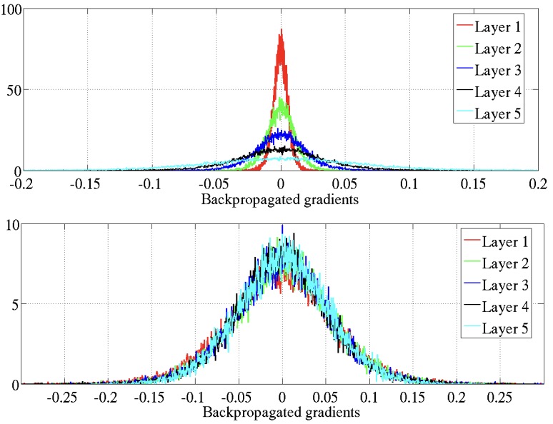
The suggested Xavier initialization \(\sigma_W^2=1/(3n)\) follows from balancing the variance of hidden layer values and the gradient to be constant through depth.
2. Random DNN Recursion Correlation Map
Let \(f_{NN}(\mathbf{x})\) denote a random Gaussian DNN: \[\mathbf{h}^{(\mathscr{l})}=W^{(\mathscr{l})}\mathbf{z}^{(\mathscr{l})}+\mathbf{b}^{(\mathscr{l})}, \mathbf{z}^{(\mathscr{l}+1)}=\phi(\mathbf{h}^{(\mathscr{l})}), \mathscr{l}=0, \ldots, L-1,\] which takes as input the vector \(\mathbf{x}\), and is parameterized by random weight matrices \(W^{(\mathscr{l})}\) and bias vectors \(\mathbf{b}^{(\mathscr{l})}\) with entries sampled i.i.d. from the Gaussian normal distribution \(\mathcal{N}(0, \sigma_W^2)\) and \(\mathcal{N}(0, \sigma_\mathbf{b}^2)\). Define the \(\mathscr{l}^2\) length of the pre-activation hidden layer \(\mathbf{h}^{(\mathscr{l})} \in \mathbb{R}^{n_\mathscr{l}}\) output as \[q^\mathscr{l}=n_\mathscr{l}^{-1}\|\mathbf{h}^{(\mathscr{l})}\|^2_{\mathscr{l}^2}:=\frac{1}{n_\mathscr{l}}\sum_{i=1}^{n_\mathscr{l}} (\mathbf{h}^{(\mathscr{l})}(i))^2,\] which is the sample mean of the random entries \((\mathbf{h}^{(\mathscr{l})}(i))^2\), each of which are identically distributed.
The norm of the hidden layer output \(q^\mathscr{l}\) has an expected value over the random draws of \(W^{(\mathscr{l})}\) and \(\mathbf{b}^{(\mathscr{l})}\) which satisfies \(\mathbb{E}[q^\mathscr{l}]=\mathbb{E}[(\mathbf{h}^{(\mathscr{l})}(i))^2]\) which as \(\mathbf{h}^{(\mathscr{l})}=W^{(\mathscr{l})}\phi(\mathbf{h}^{(\mathscr{l}-1)})+\mathbf{b}^{(\mathscr{l})}\) is \[\begin{aligned} \mathbb{E}[q^\mathscr{l}]&=\mathbb{E}[(W_i^{(\mathscr{l})}\phi(\mathbf{h}^{(\mathscr{l}-1)}))^2]+\mathbb{E}[(b_i^{(\mathscr{l})})^2] \\&=\sigma_W^2n_{\mathscr{l}-1}^{-1}\sum_{i=1}^{n_\mathscr{l}-1} \phi(h_i^{(\mathscr{l}-1)})^2+\sigma_\mathbf{b}^2 \end{aligned}\] where \(W_i^{(\mathscr{l})}\) denotes the \(i\)th row of \(W^{(\mathscr{l})}\).
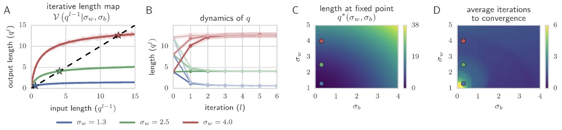
Approximating \(h_i^{(\mathscr{l}-1)}\) as Gaussian with variance \(q^{(\mathscr{l}-1)}\): \[n_{\mathscr{l}-1}^{-1}\sum_{i=1}^{n_{\mathscr{l}-1}} \phi(h_i^{(\mathscr{l}-1)})^2=\mathbb{E}[\phi(h^{(\mathscr{l}-1)})^2]=\frac{1}{\sqrt{2\pi}}\int_{-\infty}^\infty \phi\left(\sqrt{q^{(\mathscr{l}-1)}}z\right)^2e^{-z^2/2}\text{d}z\] which gives a recursive map of \(q^\mathscr{l}\) between layers \[q^{(\mathscr{l})}=\sigma_\mathbf{b}^2+\sigma_W^2\frac{1}{\sqrt{2\pi}}\int_{-\infty}^\infty \phi\left(\sqrt{q^{(\mathscr{l}-1)}}z\right)^2e^{-z^2/2}\text{d}z=:\mathcal{V}(q^{(\mathscr{l}-1)} \mid \sigma_W, \sigma_\mathbf{b}, \phi(\cdot)).\] Note that the integral is larger for \(\phi(x)=|x|\) than ReLU, which are larger than \(\phi(x)=\tanh(x)\), indicating smaller \(\sigma_W\) and \(\sigma_\mathbf{b}\) needed to ensure \(q^{(\mathscr{l})}\) has a finite nonzero limit \(q^*\). As Figure 3 shown, the fixed points are all stable.
A single input \(\mathbf{x}\) has hidden pre-activation output converging to a fixed expected length. Consider the map governing the angle between the hidden layer pre-activations of two distinct inputs \(\mathbf{x}^{(0, a)}\) and \(\mathbf{x}^{(0, b)}\): \[q_{ab}^{(\mathscr{l})}=n_\mathscr{l}^{-1}\sum_{i=1}^{n_\mathscr{l}} h_i^{(\mathscr{l})}(\mathbf{x}^{(0, a)})h_i^{(\mathscr{l})}(\mathbf{x}^{(0, b)}).\] Replacing the average in the sum with the expected values gives \[q_{ab}^{(\mathscr{l})}=\sigma_\mathbf{b}^2+\sigma_W^2\mathbb{E}[\phi(\mathbf{h}^{(\mathscr{l}-1)}(\mathbf{x}^{(0, a)}))\phi(\mathbf{h}^{(\mathscr{l}-1)}(\mathbf{x}^{(0, b)}))]\] where as before, \(h_i^{(\mathscr{l}-1)}\) is well modeled as being Gaussian with expected length \(q^{(\mathscr{l}-1)}\) which converges to fix points \(q^*\).
Define the angle between the hidden layers as \(c^{(\mathscr{l})}=q_{12}^{(\mathscr{l})}/q^*\). Writing the expectation as integral, we have \[c^{(\mathscr{l})}=\mathcal{C}(c^{(\mathscr{l}-1)} \mid \sigma_W, \sigma_\mathbf{b}, \phi(\cdot)):=\sigma_\mathbf{b}^2+\sigma_W^2\iint \text{D}z_1\text{D}z_2\phi(u_1)\phi(u_2)\] where \(\text{D}z=(2\pi)^{-1/2}e^{-z^2/2}\text{d}z\), \(u_1=\sqrt{q^*}z_1\) and \(u_2=\sqrt{q^*}\left(c^{(\mathscr{l}-1)}z_1+\sqrt{1-(c^{(\mathscr{l}-1)})^2}z_2\right)\). Normalizing by \(q^*\), we have the correlation map \[\rho^{(\mathscr{l}+1)}=c^{(\mathscr{l}+1)}:=R(\rho^{(\mathscr{l})}; \sigma_W, \sigma_\mathbf{b}, \phi(\cdot)),\] where \(R(\rho)\) measures how the correlation between two inputs evolve through the layers. By construction \(R(1)=1\) as \(c^{(\mathscr{l})} \to q^*\) as the two inputs converge to one another.
For \(\sigma_\mathbf{b}^2>0\), the correlation map satisfies \(R(0)>0\), orthogonal \(\mathbf{x}^{(0, a)}\) and \(\mathbf{x}^{(0, b)}\) become increasingly correlated with depth.
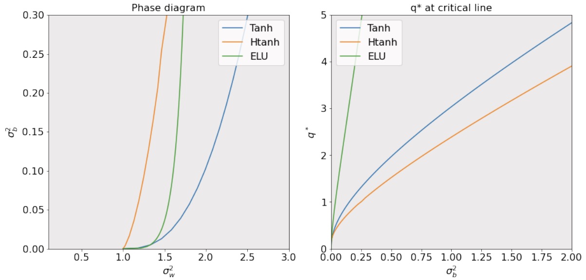
The stability of a point and its perturbation is determined by the slope of \(R(\cdot)\) at \(\rho=1\) is \[\chi:=\frac{\partial R(\rho)}{\partial \rho}\bigg|_{\rho=1}=\frac{\partial \rho^{(\mathscr{l})}}{\partial \rho^{(\mathscr{l}-1)}}\bigg|_{\rho=1}=\sigma_W^2\int \text{D}z\left[\phi'\left(\sqrt{q^*}z\right)^2\right].\] Stability of the fixed point at \(\rho=1\) is determined by \(\chi\): if \(\chi<1\), \(\rho=1\) is locally stable and points which are sufficiently correlated all converge, with depth, to the same point; if \(\chi>1\), \(\rho=1\) is unstable and nearby points become uncorrelated with depth; it is preferable to choose \(\chi=1\) if possible for \((\sigma_W, \sigma_\mathbf{b}, \phi(\cdot))\).
As Figure 4 shown, initialization on the curve allows training very deep networks.
3. Spectrum of the Jacobian
3.1. DNN Jacobian
The Jacobian is given by \[J=\frac{\partial \mathbf{z}^{(\mathscr{l})}}{\partial \mathbf{x}^{(0)}}=\prod_{\mathscr{l}=0}^{L-1} D^{(\mathscr{l})}W^{(\mathscr{l})}\] where \(D^{(\mathscr{l})}\) is diagonal with entries \(D_{ii}^{(\mathscr{l})}=\phi'(h_i^{(\mathscr{l})})\).
The Jacobian can bound the local stability of the DNN: \[\|H(\mathbf{x}+\varepsilon; \theta)-H(\mathbf{x}; \theta)\|=\|J\varepsilon+\mathcal{O}(\|\varepsilon\|^2)\| \leq \|\varepsilon\| \cdot \max\|J\|.\]
For the sum of squares loss \(\mathcal{L}\), the gradient is computed as \[\delta_\mathscr{l}=D^\mathscr{l}(W^{(\mathscr{l})})^\top\delta_{\mathscr{l}+1} \quad \text{and} \quad \delta_L=D^{(\mathscr{l})}\nabla_{\mathbf{h}^{(\mathscr{l})}}\mathcal{L}\] which gives the formula for computing the \(\delta_\mathscr{l}\) for each layer as \[\delta_\mathscr{l}=\left(\prod_{k=\mathscr{l}}^{L-1} D^{(k)}(W^{(k)})^\top\right)D^{(\mathscr{l})}\nabla_{\mathbf{h}^{(\mathscr{l})}}\mathcal{L}\] and the resulting gradient \(\nabla_\theta \mathcal{L}\) with entries as \[\frac{\partial \mathcal{L}}{\partial W^{(\mathscr{l})}}=\delta_{\mathscr{l}+1} \cdot (\mathbf{h}^{(\mathscr{l})})^\top \quad \text{and} \quad \frac{\partial \mathcal{L}}{\partial \mathbf{b}^{(\mathscr{l})}}=\delta_{\mathscr{l}+1}.\]
3.2. Stieltjes and \(\mathcal{S}\) Transform
For \(z \in \mathbb{C}-\mathbb{R}\), the Stieltjes transform \(G_\rho(z)\) of a probability distribution and its inverse are given by \[G_\rho(z)=\int_\mathbb{R} \frac{\rho(t)}{z-t}\text{d}t \quad \text{and} \quad \rho(\lambda)=-\pi^{-1}\lim_{\varepsilon \to 0_+} \text{Imag}(G_\rho(\lambda+i\varepsilon)).\] The Stieltjes transform and moment generating function are related by \[M_\rho(z):=zG_\rho(z)-1=\sum_{k=1}^\infty \frac{m_k}{z^k}\] and the \(\mathcal{S}\) transform is defined as \[S_\rho(z)=\frac{1+z}{zM_\rho^{-1}(z)}.\] The \(\mathcal{S}\) transform has the property that if \(\rho_1\) and \(\rho_2\) are freely independent, then \(S_{\rho_1\rho_2}=S_{\rho_1}S_{\rho_2}\).
The \(\mathcal{S}\) transform of \(JJ^\top\) is then given by \[\mathcal{S}_{JJ^\top}=\mathcal{S}_{D^2}^L\mathcal{S}_{W^\top W}^L,\] which can be computed through the moments \[M_{JJ^\top}(z)=\sum_{k=1}^\infty \frac{m_k}{z^k} \quad \text{and} \quad M_{D^2}(z)=\sum_{k=1}^\infty \frac{\mu_k}{z^k}\] where \(\displaystyle \mu_k=\int (2\pi)^{-1/2}\phi'\left(\sqrt{q^*}z\right)^{2k}e^{-z^2/2}\text{d}z\).
In particular, \(m_1=(\sigma_W^2\mu_1)^L\) and \(m_2=(\sigma_W^2\mu_1)^{2L}L(\mu_2^{-1}\mu_1^2+L^{-1}-1-s_1)\), where \(\sigma_W^2\mu_1=\chi\) is the growth factor we observe with the edge of chaos, requiring \(\chi=1\) to avoid rapid convergence of correlations to fixed points.
3.3. Nonlinear Activation Stability
Recall that \(m_1=\chi^L\) is the expected value of the spectrum of \(JJ^\top\), while the variance of the spectrum of \(JJ^\top\) is given by \[\sigma_{JJ^\top}^2=m_2-m_1^2=L(\mu_2\mu_1^{-2}-1-s_1)\] where for \(W\) Gaussian, \(s_1=-1\), and for \(W\) orthogonal, \(s_1=0\).
Pennington et al. (2018) found that for linear networks, the fixed point equation is \(q^*=\sigma_W^2q^*+\sigma^2_\mathbf{b}\), and \((\sigma_W, \sigma_\mathbf{b})=(1, 0)\) is the only critical point; for ReLU networks, the fixed point equation is \(\displaystyle q^*=\frac{1}{2}\sigma_W^2q^*+\sigma_\mathbf{b}^2\), and \((\sigma_W, \sigma_\mathbf{b})=(\sqrt{2}, 0)\) is the only critical point; Hard Tanh and Erf have curves as fixed points \(\chi(\sigma_W, \sigma_\mathbf{b})\).
4. Controlling the Variance of the Jacobian Spectra
Definition An activation function \(\phi: \mathbb{R} \to \mathbb{R}\) satisfying the following properties is called scaled-bounded activation:
(1) continuous;
(2) odd, i.e., \(\phi(z)=-\phi(-z)\) for all \(z \in \mathbb{R}\);
(3) linear around the origin and bounded, i.e., there exists \(a, k \in \mathbb{R}_{>0}\) s.t. \(\phi(z)=kz\) for all \(z \in [-a, a]\) and \(\phi(z) \leq ak\) for all \(z \in \mathbb{R}\);
(4) twice differentiable at all points \(z \in \mathbb{R}-\mathcal{D}\), where \(\mathcal{D} \subset \mathbb{R}\) is a finite set; furthermore \(|\phi'(z)| \leq k\) for all \(z \in \mathbb{R}-\mathcal{D}\).
Theorem (Murray et al., 2021) Let \(\phi\) be a scaled-bounded activation, \(\chi_1:=\sigma_W^2\mathbb{E}[\phi'(\sqrt{q^*}Z)^2]=1\), where \(q^*>0\) is a fixed point of \(V_\phi\), and \(\sigma_\mathbf{b}^2>0\). Let input \(\mathbf{x}\) satisfy \(\|\mathbf{x}\|_2^2=q^*\). Then as \(y:=\sigma_\mathbf{b}^2/a^2 \to 0\), \[\max_{\rho \in [0, 1]} |R_{\phi, q^*}(\rho)-\rho| \to 0 \quad \text{and} \quad |\mu_2/\mu_1^2-1| \to 0.\]
This is independent of details of \(\phi(\cdot)\) outside its linear region \([-a, a]\). Best performance is observed with \(a \sim 3\), or preferably a decreasing from about \(5\) to \(2\) during training.
5. DNN Random Initialization Summary
The hidden layers converge to fixed expected length.
Poole et al. (2016) showed pre-activation output is well modeled as Gaussian with variance \(q^*\) determined by \((\sigma_W, \sigma_\mathbf{b}, \phi(\cdot))\). Moreover, the correlation between two inputs follows a similar map with correlations converging to a fixed point, with the behavior determined in part by \(\chi\) where \(\chi=1\) avoids correlation to the same point, or nearby points diverging.
Very DNNs can be especially hard to train for activations with unfavorable initializations; e.g., ReLU with \(\chi=1\) requires \((\sigma_W, \sigma_\mathbf{b})=(\sqrt{2}, 0)\).
Pennington et al. (2018) showed more generally how to compute the moments for the Jacobian spectra, where \(\chi=1\) is needed to avoid exponential growth or shrinkage with depth of gradients.