1. Multivariate Gaussian Distribution
Definition 1.1 \(X_V\) has a multivariate Gaussian distribution with parameters \(\mu\) and \(\Sigma\) if the joint density is \[f(x_V; \mu, \Sigma)=\frac{1}{(2\pi)^{p/2}|\Sigma|^{1/2}}\exp\left[-\frac{1}{2}(x_V-\mu)^\top\Sigma^{-1}(x_V-\mu)\right],\] where \(x_V \in \mathbb{R}^p\). Note that we usually consider \[\ln f(x_V; \mu, \Sigma)=C-\frac{1}{2}(x_V-\mu)^\top\Sigma^{-1}(x_V-\mu).\] or \[\ln f(x_V; \mu, K)=C-\frac{1}{2}(x_V-\mu)^\top K(x_V-\mu).\]
Theorem 1.1 Let \(X_V\) has a multivariate Gaussian distribution with concentration matrix \(K=\Sigma^{-1}\). Then \(X_i \perp\!\!\!\!\perp X_j \mid X_{V-\{i, j\}}\) iff \(k_{ij}=0\), where \(k_{ij}\) is the corresponding entry in the concentration matrix.
2. Gaussian Graphical Model (GGM)
If \(M\) is a matrix whose rows and columns are indexed by \(A \subseteq V\), we write \(\{M\}_{A, A}\) to indicate the matrix indexed by \(V\) (i.e., it has \(|V|\) rows and columns) whose \(A, A\)-entries are \(M\) and with zeroes elsewhere. For example, if \(|V|=3\) then \[M=\begin{bmatrix}a & b \\ b & c\end{bmatrix} \quad \text{and} \quad \{M\}_{12, 12}=\begin{bmatrix}a & b & 0 \\b & c & 0 \\0 & 0 & 0\end{bmatrix},\] where \(12\) is used as an abbreviation for \(\{1, 2\}\) in the subscript.
Lemma 2.1 Let \(\mathcal{G}\) be a graph with decomposition \((A, S, B)\), and \(X_V \sim \mathcal{N}_p(0, \Sigma)\). Then \(p(x_V)\) is Markov w.r.t. \(\mathcal{G}\) iff \[\Sigma^{-1}=\{(\Sigma_{AS, AS})^{-1}\}_{AS, AS}+\{(\Sigma_{BS, BS})^{-1}\}_{BS, BS}-\{(\Sigma_{S, S})^{-1}\}_{S, S},\] and \(\Sigma_{AS, AS}\) and \(\Sigma_{BS, BS}\) are Markov w.r.t. \(\mathcal{G}_{A \cup S}\) and \(\mathcal{G}_{B \cup S}\) respectively.
Proof. Since \((A, S, B)\) is a decomposition and \(p(x_V)\) is Markov, then \(X_A \perp\!\!\!\!\perp X_B \mid X_S\), which implies for all \(x_V \in \mathbb{R}^{|V|}\), \[p(x_V)p(x_S)=p(x_A, x_S)p(x_B, x_S).\] Then \[x_V^\top\Sigma^{-1}x_V+x_S^\top(\Sigma_{S, S})^{-1}x_S=x_{AS}^\top(\Sigma_{AS, AS})^{-1}x_{AS}+x_{BS}^\top(\Sigma_{BS, BS})^{-1}x_{BS},\] i.e., \[x_V^\top\Sigma^{-1}x_V+x_V^\top\{(\Sigma_{S, S})^{-1}\}_{S, S}x_V=x_V^\top\{(\Sigma_{AS, AS})^{-1}\}_{AS, AS}x_V+x_V^\top\{(\Sigma_{BS, BS})^{-1}\}_{BS, BS}x_V.\] Therefore, \[\Sigma^{-1}=\{(\Sigma_{AS, AS})^{-1}\}_{AS, AS}+\{(\Sigma_{BS, BS})^{-1}\}_{BS, BS}-\{(\Sigma_{S, S})^{-1}\}_{S, S}.\]
The converse holds similarly.\(\square\)
3. Maximum Likelihood Estimation
Let \(X_V^{(1)}, \ldots, X_V^{(n)} \overset{\text{i.i.d.}}{\sim} \mathcal{N}_p(0, \Sigma)\). The sufficient statistic for \(\Sigma\) is the sample covariance matrix \[W=\frac{1}{n}\sum_{i=1}^n X_V^{(i)}(X_V^{(i)})^\top.\] In addition, \(\widehat{\Sigma}=W\) is the MLE for \(\Sigma\) under the unrestricted model (i.e., when all edges are present in the graph). Let \(\widehat{\Sigma}^\mathcal{G}\) denote the MLE for \(\Sigma\) under the restriction that the distribution satisfies the Markov property for \(\mathcal{G}\), and \(\widehat{K}^\mathcal{G}\) denote the inverse of \(\widehat{\Sigma}^\mathcal{G}\).
For a decomposable graph \(\mathcal{G}\) with cliques \(C_1, \ldots, C_k\), the MLE can be written in the form \[(\widehat{\Sigma}^\mathcal{G})^{-1}=\sum_{i=1}^k\{(W_{C_i, C_i})^{-1}\}_{C_i, C_i}-\sum_{i=2}^k \{(W_{S_i, S_i})^{-1}\}_{S_i, S_i}.\]
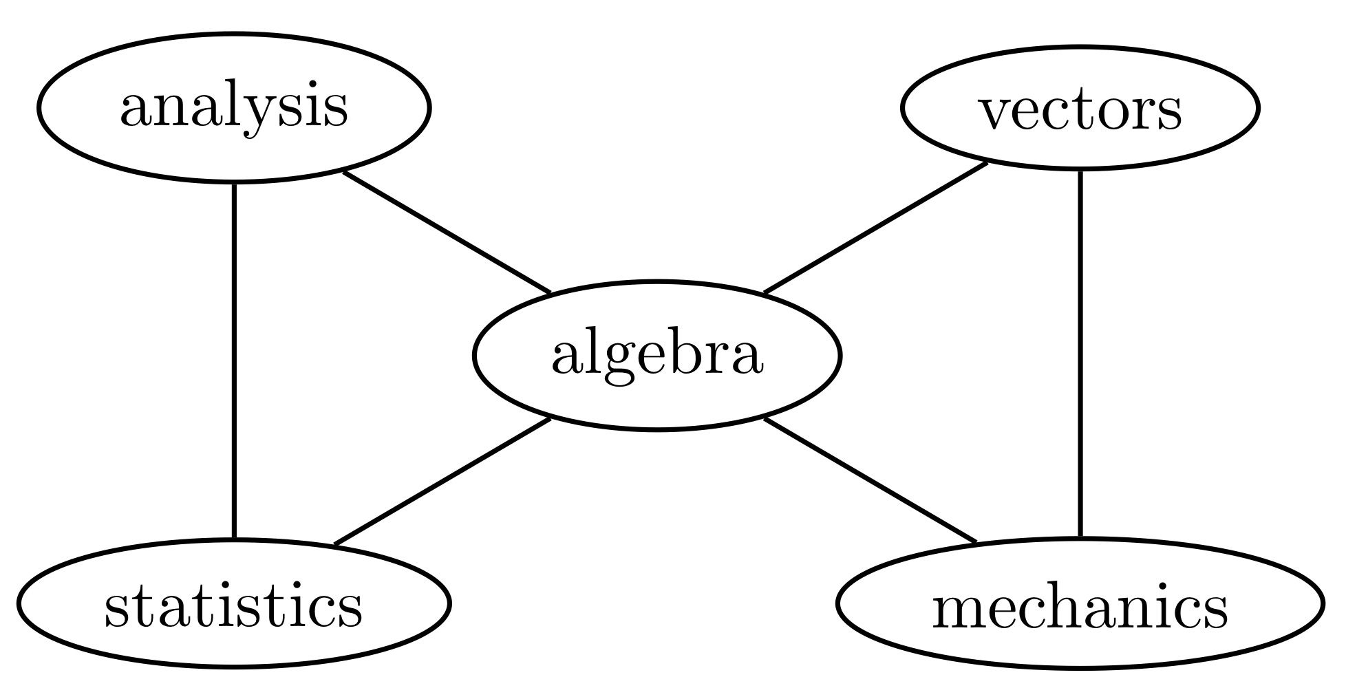
Example 3.1 Whittaker (1990) analyzed data on five maths test results administered to 88 students, in analysis, algebra, vectors, mechanics and statistics. Some of the entries in the concentration matrix are quite small, suggesting that conditional independence holds. We want to fit a graphical model and check if it gives an excellent fit.
By computation, \(\widehat{\Sigma}^\mathcal{G}\) is:
|
|
|
|
|
|
|
|---|---|---|---|---|---|
|
|
|
|
|
|
|
|
|
|
|
|
|
|
|
|
|
|
|
|
|
|
|
|
|
|
|
|
|
|
|
|
|
|
|
We carry out a likelihood ratio test to see whether this model is a good fit to the data. We want to test \[H_0: \text{Restricted model} \quad \text{against} \quad H_1: \text{Unrestricted model}.\] The test statistic is \[2(l(\widehat{\Sigma})-l(\widehat{\Sigma}^\mathcal{G}))=0.8958244 \to \chi^2_{(4)}\] and the \(p\)-value is \(0.925>0.05\), i.e., the model is a good fit.
Here is the relevant code in R:
library(ggm) |