1. Tensor

创建一个随机初始化的张量（\(5 \times 3\)矩阵）：torch.rand(5, 3).
创建一个全为\(0\)的张量（\(5 \times 3\)矩阵）：torch.zeros(5, 3, dtype=torch.long), 其中数据类型是long.
创建一个张量：torch.tensor([1.3, 1.4]).
基于已经存在的张量创建一个张量：

x = x.new_ones(5, 3, dtype=torch.double)
x = torch.randn_like(x, dtype=torch.float)

获取张量的维度信息：x.size().

2. Operation

加法的几种方式：

x = torch.rand(5, 3)
y = torch.rand(5, 3)

# 方法一
x + y

# 方法二
torch.add(x, y)
result = torch.empty(5, 3)
torch.add(x, y, out=result) # 将结果储存于result中

# 方法三
y.add_(x)

_会使张量发生变化，例如x.copy_(y)或x.t_()都会改变x.

使用torch.view改变张量的大小或形状：

x = torch.randn(6, 4)
y = x.view(24)
z = x.view(-1, 8)

view(-1, n)中-1的大小是由其它位置推断出来的，比如上例中z是一个\(3 \times 8\)的矩阵。

如果张量仅为一个元素，可以使用.item()来获得这个元素的值：

x = torch.randn(1)
x.item()

3. Automatic Differentiation

如果将torch.Tensor的属性.requires_grad设置为True, 则会开始跟踪针对张量的所有操作。在完成计算后，调用.backward()来自动计算所有梯度。张量的梯度将累积到.grad属性中。

x = torch.ones(2, 2, requires_grad=True)
y = x + 2
z = y * y * 3
out = z.mean()

out.backward()
x.grad # d(out)/dx

Let out be \(o\), then \(\displaystyle o=\frac{1}{4}\sum_i z_i\), where \(z_i=3(x_i+2)^2\). Hence, \(\displaystyle \frac{\partial o}{\partial x_i}=\frac{3}{2}(x_i+2)\), and thus \(\displaystyle \frac{\partial o}{\partial x_i}\bigg|_{x_i-1}=4.5\).

当调用.backward()时，一个张量会自动传递为.backward(torch.tensor(1.0)), 其中torch.tensor(1.0)是用来终止链式法则梯度乘法的外部梯度。

.backward()中的张量的维数必须与正在计算梯度的张量的维数相同：

x = torch.tensor([0., 2., 8.], requires_grad=True)
y = torch.tensor([5., 9., 7.], requires_grad=True)
z = x * y

z.backward() # RuntimeError: grad can be implicitly created only for scalar outputs
z.backward(torch.tensor([1., 1., 1.]))
x.grad # tensor([5., 9., 7.])
y.grad # tensor([0., 2., 8.])

Tensor和Function互相连接并构建一个保存整个完整计算过程的历史信息的非循环图。每一个张量都一个.grad_fn属性，这一属性保存着创建张量的Function的引用。如果是用户自己创建张量，则.grad_fn为None:

x = torch.ones(2, 2, requires_grad=True)
print(x.grad_fn) # None

y = x + 2
print(y.grad_fn) # <AddBackward0 object at 0x7fe7900ccd00>

如果要停止张量历史记录的跟踪，调用.detach()来将其与计算历史记录分离，并防止将来的计算被跟踪。此外，还可以使用with torch.no_grad():包装起来——在评估模型时尤其有用，因为模型在训练阶段具有requires_grad=True的可训练参数有利于有利于调参，但在评估阶段我们不需要梯度。
.requires_grad_()会改变张量的requires_grad标记。如果没有提供相应的参数，输入的标记默认为False.

4. Neural Network

一个典型的神经网络训练过程包括：

定义一个包含可训练参数的神经网络。
迭代整个输入。
通过神经网络处理输入。
计算损失。
反向传播梯度到神经网络的参数。
更新网络的参数。

4.1. Example: LeNet-5

考虑一个简单的前馈神经网络。

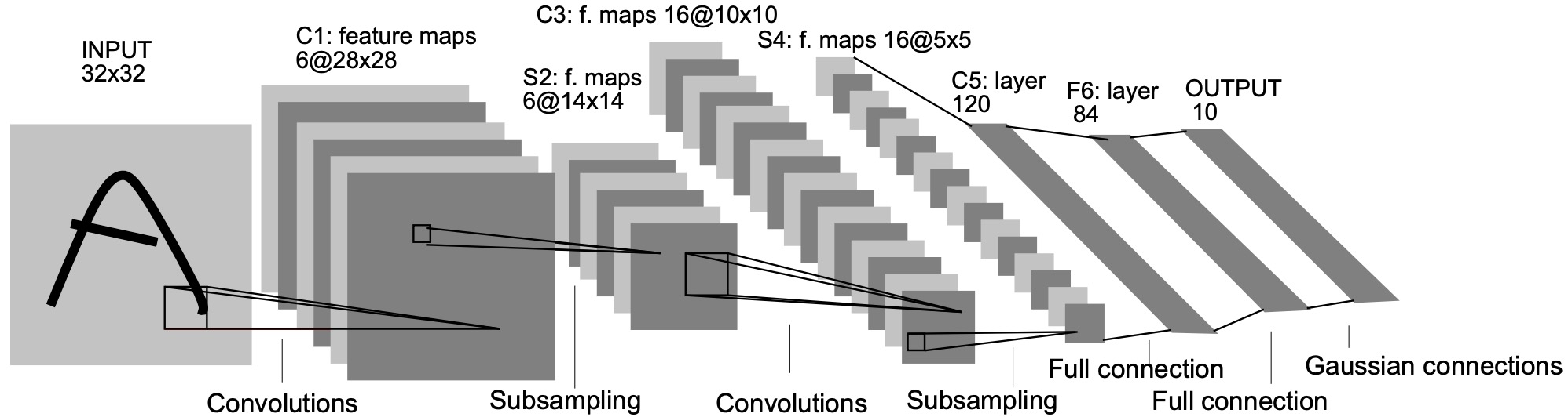
Figure 1: Architecture of LeNet-5 (LeCun et al., 1998). LeNet-5神经网络一共五层，其中卷基层和池化层可以考虑为一个整体。网络的结构为：输入 \(\to\) 卷积 \(\to\) 池化 \(\to\) 卷积 \(\to\) 池化 \(\to\) 全连接 \(\to\) 全连接 \(\to\) 全连接 \(\to\) 输出

在PyTorch中，图像数据集的存储顺序为(batch, channels, height, width)，依次为批大小、通道数、高度、宽度。按照网络结构，我们可以整理得：

Table 1: Parameters of LeNet-5.

操作	操作参数	输入/输出尺寸
`input`	`channels=1` `height=32` `width=32`	Input: `(b, 1, 32, 32)` Output: `(b, 1, 32, 32)`
`conv1`	`in_channels=1` `out_channels=6` `kernel_size=5` `padding=0` `stride=1`	Input: `(b, 1, 32, 32)` Output: `(b, 6, 28, 28)`
`pool1`	`kernel_size=2`	Input: `(b, 6, 28, 28)` Output: `(b, 6, 14, 14)`
`conv2`	`in_channels=6` `out_channels=16` `kernel_size=5` `padding=0` `stride=1`	Input: `(b, 6, 14, 14)` Output: `(b, 16, 10, 10)`
`pool2`	`kernel_size=2`	Input: `(b, 16, 10, 10)` Output: `(b, 16, 5, 5)`
`fc1`	`in=1655` `out=120`	Input: `(b, 1655)` Output: `(b, 120)`
`fc2`	`in=120` `out=84`	Input: `(b, 120)` Output: `(b, 84)`
`fc3`	`in=84` `out=10`	Input: `(b, 84)` Output: `(b, 10)`

4.1.1. torch.nn.Conv2d

卷积层用于提取特征。torch.nn.Conv2d是二维卷积方法（常用于二维图像），相对应的还有一维卷积方法torch.nn.Conv1d（常用于文本数据的处理）。torch.nn.Conv2d有9个参数，我们先介绍6个较为重要的参数：

in_channels及out_channels: channels意为通道数。在输入层中的RGB图片，channels=3（红、绿、蓝）；而单色图，channels=1. 一般而言，channels指每个卷基层中卷积核的数量。
kernel_size: 卷积核的大小，可以用int表示长宽相等的卷积核，或者用tuple.表示长宽不同的卷积核。
stride: 步长，用来控制卷积核移动间隔，默认stride=1.
padding: 填充宽度。例如当padding=1的时候，如果原来的大小为\(3 \times 3\), 那么填充后的大小为\(5 \times 5\), 即在外围加了一圈, 默认padding=0.
padding_mode: 填充宽度的方式，默认padding_mode="zeros".

4.1.2. torch.nn.MaxPool2d

池化层用于提取重要信息，可以去掉不重要的信息，减少计算开销。torch.nn.MaxPool2d在提取数据时，保留相邻信息中的最大值，并去掉其它值。我们先介绍torch.nn.MaxPool2d中2个较为重要的参数：

kernel_size: 池化核的大小，与卷积核类似。
stride: 步长，默认stride=kernel_size`.

4.1.3. torch.nn.Linear

torch.nn.Linear用于设置网络中的全连接层。在二维图像处理的任务中，全连接层的输入与输出一般都设置为二维张量(batch, size). torch.nn.Linear有三个参数，分别为in_features, out_features和bias.

4.2. Code

神经网络可以通过torch.nn来构建。首先我们定义图片中的神经网络：

import torch
import torch.nn as nn
import torch.nn.functional as F

class LeNet5(nn.Module):
    def __init__(self):
        super(LeNet5, self).__init__()
        self.conv1 = nn.Conv2d(in_channels=1, out_channels=6, kernel_size=5)
        self.pool1 = nn.MaxPool2d(2)
        self.conv2 = nn.Conv2d(6, 16, 5)
        self.pool2 = nn.MaxPool2d(2)
        self.fc1 = nn.Linear(16*5*5, 120)
        self.fc2 = nn.Linear(120, 84)
        self.fc3 = nn.Linear(84, 10)
        
    def forward(self, x):
        x = self.pool1(F.relu(self.conv1(x)))
        x = self.pool2(F.relu(self.conv2(x)))
        x = x.view(x.size()[0], -1)
        x = F.relu(self.fc1(x))
        x = F.relu(self.fc2(x))
        x = self.fc3(x)
        return x

一个模型可训练的参数可以通过调用LeNet5.parameters()返回。
一个简单的损失函数是均方误差nn.MSELoss(output, target).
调用LeNet5.zero_grad()将梯度清零，并随机的梯度来反向传播loss.vackward().
利用梯度更新神经网络，最简单的更新规则是随机梯度下降：

learning_rate = 0.01
for f in LeNet5.parameters():
    f.data.sub_(f.grad.data * learning_rate)

此外，我们可以使用不同的更新规则，比如Adam等：

import torch.optim as optim

optimizer = optim.SGD(LeNet5.parameters(), lr=0.01)

# 训练过程循环：
optimizer.zero_grad()
output = LeNet5(input)
loss = nn.MSELoss(output, target)
loss.backward()
optimizer.step()

5. Reference

Yann LeCun, Leon Bottou, Yoshua Bengio, and Patrick Haffner. Gradient-Based Learning Applied to Document Recognition. Proceedings of the IEEE, 86(11): 2278-2324, 1998.

Tianyang Li

Introduction to PyTorch