1. Preliminary
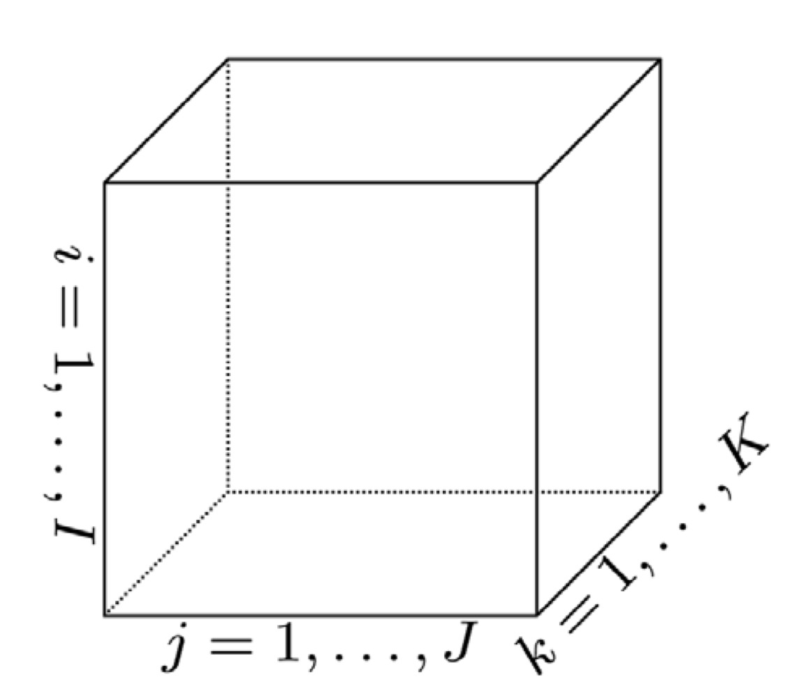
A tensor is a multidimensional array. A first-order tensor is a vector, a second-order tensor is a matrix, and tensor of order three or higher are called higher-order tensor. A third-order tensor has three indices:
1.1. Fibers
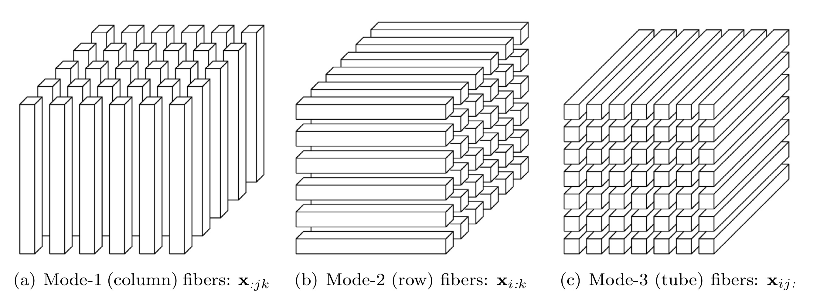
Fibers are the higher-order analogue of matrix rows and columns, defined by fixing every index but one. A matrix column is a mode-\(1\) fiber and a matrix row is a mode-\(2\) fiber. Third-order tensor \(\mathbfcal{X}\) has column, row and tube fibers, denoted by \(\mathbf{x}_{:jk}\), \(\mathbf{x}_{i:k}\) and \(\mathbf{x}_{ij:}\), respectively.
当一个张量沿着第\(k\)维展开时,我们就得到了mode-\(k\) fiber.
1.2. Slices
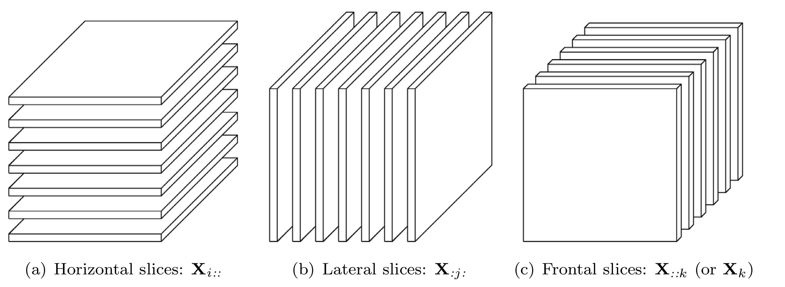
Slices are two-dimensional sections of a tensor, defined by fixing all but two indices. Third-order tensor \(\mathbfcal{X}\) has horizontal, lateral and frontal slides, denoted by \(\mathbf{X}_{i::}\), \(\mathbf{X}_{:j:}\) and \(\mathbf{X}_{::k}\), respectively. The \(k\)th frontal slice of a third-order tensor may be denoted more compactly as \(\mathbf{X}_k\).
1.3. Norm
The norm of a tensor \(\mathbfcal{X} \in \mathbb{R}^{I_1 \times \cdots \times I_N}\) is the square root of the sum of the squares of all its entries: \[\|\mathbfcal{X}\|=\sqrt{\sum_{i_1=1}^{I_1} \cdots \sum_{i_N=1}^{I_N} x_{i_1, \ldots, x_N}^2}.\]
1.4. Inner Product
The inner product of two same-sized tensors \(\mathbfcal{X}, \mathbfcal{Y} \in \mathbb{R}^{I_1 \times \cdots \times I_N}\) is the sum of the products of their entries: \[\langle \mathbfcal{X}, \mathbfcal{Y} \rangle=\sum_{i_1=1}^{I_1} \cdots \sum_{i_N=1}^{I_N} x_{i_1, \ldots, x_N}y_{i_1, \ldots, x_N}\] which follows immediately that \(\langle \mathbfcal{X}, \mathbfcal{X} \rangle=\|\mathbfcal{X}\|^2\).
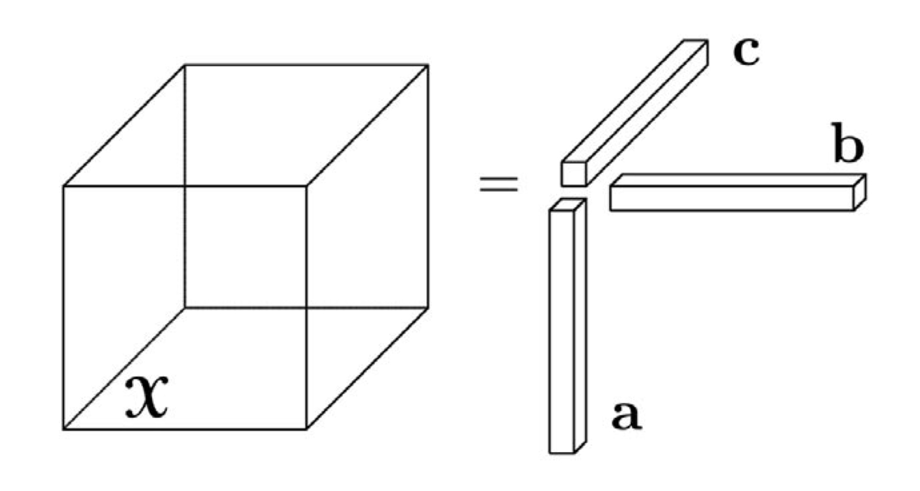
1.5. Rank-One Tensor
An \(N\)th-order tensor \(\mathbfcal{X} \in \mathbb{R}^{I_1 \times \cdots \times I_N}\) is rank-one if it can be written as the outer product of \(N\) vectors: \[\mathbfcal{X}=\mathbf{a}^{(1)} \circ \cdots \circ \mathbf{a}^{(N)}.\] The symbol \(\circ\) represents the vector outer product, which means that each element of the tensor is the product of the corresponding vector elements, i.e., for all \(1 \leq i_n \leq I_n\), \[x_{i_1, \ldots, i_N}=a_{i_1}^{(1)} \cdots a_{i_N}^{(N)}.\]
1.6. Symmetry
A tensor is called cubical if every mode is the same size, i.e., \(\mathbfcal{X} \in \mathbb{R}^{I \times \cdots \times I}\). A cubical tensor is called supersymmetric if its elements remain constant under any permutation of the indices. For instance, a third-order tensor \(\mathbfcal{X} \in \mathbb{R}^{I \times I \times I}\) is supersymmetric if for all \(i, j, k=1, \ldots, I\), \[x_{ijk}=x_{ikj}=x_{jik}=x_{jki}=x_{kij}=x_{kji}.\]
Tensor can be partially symmetric in two or more modes. For instance, a third-order tensor \(\mathbfcal{X} \in \mathbb{R}^{I \times I \times K}\) is symmetric in modes one and two if all its frontal slices are symmetric, i.e., for all \(k=1, \ldots, K\), \[\mathbf{X}_k=\mathbf{X}_k^\top.\]
张量在mode-\(1\)和\(2\)下对称,可以理解为展开第\(1\)维和第\(2\)维,固定剩余维度的情况下,所获得的slice是对称的。
1.7. Diagonal Tensor
A tensor \(\mathbfcal{X} \in \mathbb{R}^{I_1 \times \cdots \times I_N}\) is diagonal if \(x_{i_1, \ldots, i_N} \neq 0\) only if \(i_1=\cdots=i_N\).
1.8. Matricization: Transforming a Tensor into a Matirx
Matricization, a.k.a. unfolding or flattening, is the process of reordering the elements of an \(N\)th-order tensor into a matrix. For example, a \(2 \times 3 \times 4\) tensor can be arranged as a \(6 \times 4\) matrix or a \(3 \times 8\) matrix.
The mode-\(n\) matricization of a tensor \(\mathbfcal{X} \in \mathbb{R}^{I_1 \times \cdots \times I_N}\) is denoted by \(\mathbf{X}_{(n)}\) and arranges the mode-\(n\) fibers to be the columns of the resulting matrix. Mathematically, tensor element \((i_1, \ldots, i_N)\) maps to matrix element \((i_n, j)\), where \(\displaystyle j=1+\sum_{\substack{k=1 \\ k \neq n}}^N (i_k-1)J_k\) and \(\displaystyle J_k=\prod_{\substack{m=1 \\m \neq n}}^{k-1} I_m\).
Example 1.1 Let the frontal slices of \(\mathbfcal{X} \in \mathbb{R}^{3 \times 4 \times 2}\) be \[\mathbf{X}_1=\begin{bmatrix} 1 & 4 & 7 & 10 \\ 2 & 5 & 8 & 11 \\ 3 & 6 & 9 & 12 \end{bmatrix} \quad \text{and} \quad \mathbf{X}_2=\begin{bmatrix} 13 & 16 & 19 & 22 \\ 14 & 17 & 20 & 23 \\ 15 & 18 & 21 & 24 \end{bmatrix}.\] Then the three mode-\(n\) unfoldings are \[\mathbf{X}_{(1)}=\begin{bmatrix} 1 & 4 & 7 & 10 & 13 & 16 & 19 & 22 \\ 2 & 5 & 8 & 11 & 14 & 17 & 20 & 23 \\ 3 & 6 & 9 & 12 & 15 & 18 & 21 & 24 \\ \end{bmatrix},\] \[\mathbf{X}_{(2)}=\begin{bmatrix} 1 & 2 & 3 & 13 & 14 & 15 \\ 4 & 5 & 6 & 16 & 17 & 18 \\ 7 & 8 & 9 & 19 & 20 & 21 \\ 10 & 11 & 12 & 22 & 23 & 24 \end{bmatrix},\] and
\[\mathbf{X}_{(3)}=\begin{bmatrix} 1 & 2 & 3 & 4 & \cdots & 9 & 10 & 11 & 12 \\ 13 & 14 & 15 & 16 & \cdots & 21 & 22 & 23 & 24 \\ \end{bmatrix}.\]
不同的论文有时在展开时使用完全不同的排序方法,只要这些排序方法是前后一致的,一般来说不会给理论或计算带来影响。
1.9. The \(n\)-Mode Product
The \(n\)-mode matrix product of a tensor \(\mathbfcal{X} \in \mathbb{R}^{I_1 \times \cdots \times I_N}\) with a matrix \(\mathbf{U} \in \mathbb{R}^{J \times I_n}\) is denoted by \(\mathbfcal{X} \times_n \mathbf{U}\) and is of size \(I_1 \times \cdots \times I_{n-1} \times J \times I_{n+1} \times \cdots I_N\). Elementwise, we have \[(\mathbfcal{X} \times_n \mathbf{U})_{i_1, \ldots, i_{n-1}, j, i_{n+1}, \ldots, i_N}=\sum_{i_n=1}^{I_n} x_{i_1, \ldots, i_N}u_{j, i_n}.\] Each mode-\(n\) fiber is multiplied by the matrix \(\mathbf{U}\), and it can also be expressed in terms of unfolded tensors \[\mathbfcal{Y}=\mathbfcal{X} \times_n \mathbf{U} \Leftrightarrow \mathbf{Y}_{(n)}=\mathbf{U}\mathbf{X}_{(n)}.\]
Example 1.2 Let the frontal slices of \(\mathbfcal{X} \in \mathbb{R}^{3 \times 4 \times 2}\) be \[\mathbf{X}_1=\begin{bmatrix} 1 & 4 & 7 & 10 \\ 2 & 5 & 8 & 11 \\ 3 & 6 & 9 & 12 \end{bmatrix} \quad \text{and} \quad \mathbf{X}_2=\begin{bmatrix} 13 & 16 & 19 & 22 \\ 14 & 17 & 20 & 23 \\ 15 & 18 & 21 & 24 \end{bmatrix}.\] Let \(\mathbf{U}=\begin{bmatrix} 1 & 3 & 5 \\ 2 & 4 & 6 \end{bmatrix}\), then \(\mathbfcal{Y}=\mathbfcal{X} \times_1 \mathbf{U} \in \mathbb{R}^{2 \times 4 \times 2}\) with \[\mathbf{Y}_1=\begin{bmatrix} 22 & 49 & 76 & 103 \\ 28 & 64 & 100 & 136 \\ \end{bmatrix} \quad \text{and} \quad \mathbf{Y}_2=\begin{bmatrix} 130 & 157 & 184 & 211 \\ 172 & 208 & 244 & 280 \end{bmatrix}.\]
For distinct modes in a series of multiplications, the order of the multiplication is irrelevant, i.e., for \(m \neq n\), \[\mathbfcal{X} \times_m \mathbf{A} \times_n \mathbf{B}=\mathbfcal{X} \times_n \mathbf{B} \times_m \mathbf{A}.\] If the modes are the same, then \[\mathbfcal{X} \times_n \mathbf{A} \times_n \mathbf{B}=\mathbfcal{X} \times_n (\mathbf{BA}).\]
The \(n\)-mode vector product of a tensor \(\mathbfcal{X} \in \mathbb{R}^{I_1 \times \cdots I_N}\) with a vector \(\mathbf{v} \in \mathbb{R}^{I_n}\) is denoted by \(\mathbfcal{X} \overline{\times}_n \mathbf{v}\). The result is of order \(N-1\), i.e., the size is \(I_1 \times \cdots \times I_{n-1} \times I_{n+1} \times \cdots \times I_N\). Elementwise, we have \[(\mathbfcal{X} \overline{\times}_n \mathbf{v})_{i_1, \ldots, i_{n-1}, i_{n+1}, \ldots, i_N}=\sum_{i_n=1}^{I_n} x_{i_1, \ldots, i_N}v_{i_n}.\] The idea is to compute the inner product of each mode-\(n\) fiber with the vector \(\mathbf{v}\).
Example 1.3 Let the frontal slices of \(\mathbfcal{X} \in \mathbb{R}^{3 \times 4 \times 2}\) be \[\mathbf{X}_1=\begin{bmatrix} 1 & 4 & 7 & 10 \\ 2 & 5 & 8 & 11 \\ 3 & 6 & 9 & 12 \end{bmatrix} \quad \text{and} \quad \mathbf{X}_2=\begin{bmatrix} 13 & 16 & 19 & 22 \\ 14 & 17 & 20 & 23 \\ 15 & 18 & 21 & 24 \end{bmatrix}.\] Let \(\mathbf{v}=\begin{bmatrix} 1 \\ 2 \\ 3 \\ 4 \end{bmatrix}\), then \(\mathbfcal{X} \overline{\times}_2 \mathbf{v}=\begin{bmatrix} 70 & 190 \\ 80 & 200 \\ 90 & 210 \end{bmatrix}\).
When it comes to mode-\(n\) vector multiplication, precedence matters because the order of the intermediate results changes, i.e., for \(m<n\), \[\mathbfcal{X} \overline{\times}_m \mathbf{a} \overline{\times}_n \mathbf{b}=(\mathbfcal{X} \overline{\times}_m \mathbf{a}) \overline{\times}_{n-1} \mathbf{b}=(\mathbfcal{X} \overline{\times}_n \mathbf{b}) \overline{\times}_m \mathbf{a}.\]
1.10. Special Matrix Product
1.10.1. Kronecker Product
Suppose \(\mathbf{A} \in \mathbb{R}^{I \times J}\) and \(\mathbf{B} \in \mathbb{R}^{K \times L}\), then \(\mathbf{A} \otimes \mathbf{B} \in \mathbb{R}^{(IK) \times (JL)}\), where \[\mathbf{A} \otimes \mathbf{B}=\begin{bmatrix} a_{11}\mathbf{B} & a_{12}\mathbf{B} & \cdots & a_{1J}\mathbf{B} \\ a_{21}\mathbf{B} & a_{22}\mathbf{B} & \cdots & a_{2J}\mathbf{B} \\ \vdots & \vdots & \ddots & \vdots \\ a_{I1}\mathbf{B} & a_{I2}\mathbf{B} & \cdots & a_{IJ}\mathbf{B} \end{bmatrix}=\begin{bmatrix} &\\ \mathbf{a}_1 \otimes \mathbf{b}_1 & \mathbf{a}_1 \otimes \mathbf{b}_2 & \cdots \mathbf{a}_J \otimes \mathbf{b}_{L-1} & \mathbf{a}_n \otimes \mathbf{b}_L \\ & \end{bmatrix}.\]
Example 1.4 Suppose \(\mathbf{A}=\begin{bmatrix} 1 & 3 \\ 2 & 4 \end{bmatrix}\) and \(\mathbf{B}=\begin{bmatrix} 5 & 7 \\ 6 & 8 \end{bmatrix}\), then \(\mathbf{A} \otimes \mathbf{B}=\begin{bmatrix} 5 & 7 & 15 & 21 \\ 6 & 8 & 18 & 24 \\ 10 & 14 & 20 & 28 \\ 12 & 16 & 24 & 32 \end{bmatrix}\).
Example 1.5 Suppose \(\mathbf{a}=\begin{bmatrix} 1 & 2 \end{bmatrix}\) and \(\mathbf{b}=\begin{bmatrix} 7 & 8 \end{bmatrix}\), then \(\mathbf{a} \otimes \mathbf{b}=\begin{bmatrix} 7 & 8 & 14 & 16 \end{bmatrix}\).
Example 1.6 Suppose \(\mathbf{a}=\begin{bmatrix} 1 & 2 \end{bmatrix}\) and \(\mathbf{b}=\begin{bmatrix} 7 \\ 8 \end{bmatrix}\), then \(\mathbf{a} \otimes \mathbf{b}=\begin{bmatrix} 7 & 14 \\ 8 & 16 \end{bmatrix}\).
1.10.2. Khatri–Rao Product
Khatri–Rao product is the matching columnwise Kronecker product. Suppose \(\mathbf{A} \in \mathbb{R}^{I \times K}\) and \(\mathbf{B} \in \mathbb{R}^{J \times K}\), then \(\mathbf{A} \odot \mathbf{B} \in \mathbb{R}^{(IJ) \times K}\), where \[\mathbf{A} \odot \mathbf{B}=\begin{bmatrix} &\\ \mathbf{a}_1 \otimes \mathbf{b}_1 & \mathbf{a}_2 \otimes \mathbf{b}_2 & \cdots \mathbf{a}_{K-1} \otimes \mathbf{b}_{K-1} & \mathbf{a}_K \otimes \mathbf{b}_K \\ & \end{bmatrix}.\]
Example 1.7 Suppose \(\mathbf{A}=\begin{bmatrix} 1 & 3 \\ 2 & 4 \end{bmatrix}\) and \(\mathbf{B}=\begin{bmatrix} 5 & 7 \\ 6 & 8 \end{bmatrix}\), then \(\mathbf{A} \odot \mathbf{B}=\begin{bmatrix} 5 & 21 \\ 6 & 24 \\ 10 & 28 \\ 12 & 32 \end{bmatrix}\).
If \(\mathbf{a}\) and \(\mathbf{b}\) are vectors, then Khatri-Rao product and Kronecker product are identical, i.e., \(\mathbf{a} \otimes \mathbf{b}=\mathbf{a} \odot \mathbf{b}\).
1.10.3. Hadamard Product
Hadamard product is the elementwise matrix product. Suppose \(\mathbf{A} \in \mathbb{R}^{I \times J}\) and \(\mathbf{B} \in \mathbb{R}^{I \times J}\), then \(\mathbf{A} * \mathbf{B} \in \mathbb{R}^{I \times J}\), where \[\mathbf{A} * \mathbf{B}=\begin{bmatrix} a_{11}b_{11} & \cdots & a_{1J}b_{1J} \\ \vdots & & \vdots \\ a_{I1}b_{I1} & \cdots & a_{IJ}b_{IJ} \end{bmatrix}.\]
1.10.4. Property
\((\mathbf{A} \otimes \mathbf{B})(\mathbf{C} \otimes \mathbf{D})=\mathbf{AC} \otimes \mathbf{BD}\).
\((\mathbf{A} \otimes \mathbf{B})^\dagger=\mathbf{A}^\dagger \otimes \mathbf{B}^\dagger\), where \(\mathbf{A}^\dagger\) denotes the Moore-Penrose pseudo-inverse of \(\mathbf{A}\).
\(\mathbf{A} \odot \mathbf{B} \odot \mathbf{C}=(\mathbf{A} \odot \mathbf{B}) \odot \mathbf{C}=\mathbf{A} \odot (\mathbf{B} \odot \mathbf{C})\).
\((\mathbf{A} \odot \mathbf{B})^\top(\mathbf{A} \odot \mathbf{B})=\mathbf{A}^\top\mathbf{A}*\mathbf{B}^\top\mathbf{B}\).
\((\mathbf{A} \odot \mathbf{B})^\dagger=((\mathbf{A}^\top\mathbf{A}) * (\mathbf{B}^\top\mathbf{B}))^\dagger(\mathbf{A} \odot \mathbf{B})^\top\).
Example 1.8 Let \(\mathbfcal{X} \in \mathbb{R}^{I_1 \times \cdots \times I_N}\) and \(\mathbf{A}^{(n)} \in \mathbb{R}^{J_n \times I_n}\) for all \(n \in \{1, \ldots, N\}\). Then for any \(n\), \[\begin{aligned} \mathbfcal{Y}&=\mathbfcal{X} \times_1 \mathbf{A}^{(1)} \times_2 \mathbf{A}^{(2)} \times_3 \cdots \times_N \mathbf{A}^{(N)} \\\Leftrightarrow \mathbf{Y}_{(n)}&=\mathbf{A}^{(n)}\mathbf{X}_{(n)}(\mathbf{A}^{(N)} \otimes \cdots \otimes \mathbf{A}^{(n+1)} \otimes \mathbf{A}^{(n-1)} \otimes \cdots \otimes \mathbf{A}^{(1)})^\top. \end{aligned}\]
2. Tensor Rank and CANDECOMP/PARAFAC Decomposition
2.1. CANDECOMP/PARAFAC (CP) Decomposition
We refer to the CANDECOMP/PARAFAC decomposition as CP. The CP decomposition factorizes a tensor into a sum of component rank-one tensors.
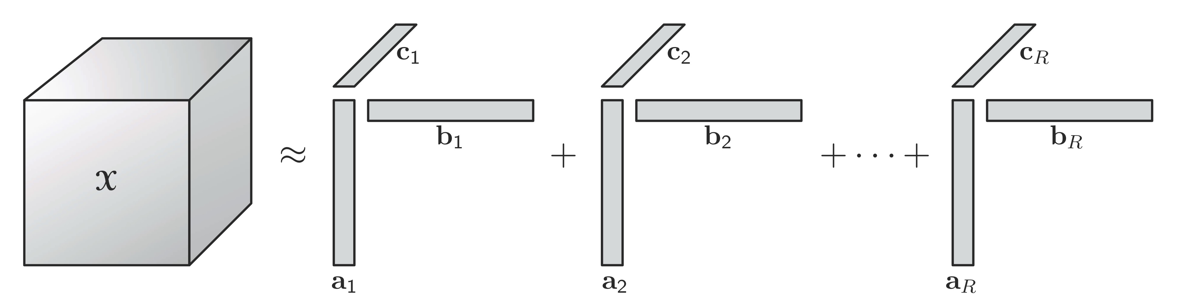
For example, given a third-order tensor \(\mathbfcal{X} \in \mathbb{R}^{I \times J \times K}\), \[\mathbfcal{X} \approx \sum_{r=1}^R \mathbf{a}_r \circ \mathbf{b}_r \circ \mathbf{c}_r,\] where \(R\) is a positive integer and \(\mathbf{a}_r \in \mathbb{R}^I\), \(\mathbf{b}_r \in \mathbb{R}^J\), and \(\mathbf{c}_r \in \mathbb{R}^K\) for \(r=1, \ldots, R\). Elementwise, for \(i=1, \ldots, I\), \(j=1, \ldots, J\), and \(k=1, \ldots, K\), \[x_{ijk} \approx \sum_{r=1}^R a_{ir}b_{jr}c_{kr}.\]
The factor matrix refers to the combination of the vectors from the rank-one components. For example, \(\mathbf{A}=\begin{bmatrix} & \\ \mathbf{a}_1 & \cdots & \mathbf{a}_R \\ & \end{bmatrix}.\) With the definition, we can write the CP decomposition in matricized form (one per mode): \[\begin{aligned} \mathbf{X}_{(1)} &\approx \mathbf{A}(\mathbf{C} \odot \mathbf{B})^\top, \\ \mathbf{X}_{(2)} &\approx \mathbf{B}(\mathbf{C} \odot \mathbf{A})^\top, \\ \mathbf{X}_{(3)} &\approx \mathbf{C}(\mathbf{B} \odot \mathbf{A})^\top. \end{aligned}\]
The CP model can be concisely expressed as \[\mathbfcal{X} \approx [\![\mathbf{A}, \mathbf{B}, \mathbf{C}]\!]=\sum_{r=1}^R \mathbf{a}_r \circ \mathbf{b}_r \circ \mathbf{c}_r.\] It is often useful to assume that the columns of \(\mathbf{A}\), \(\mathbf{B}\) and \(\mathbf{C}\) are normalized to length \(1\) with the weights absorbed into the vector \(\boldsymbol{\lambda} \in \mathbb{R}^R\) so that \[\mathbfcal{X} \approx [\![\boldsymbol{\lambda}; \mathbf{A}, \mathbf{B}, \mathbf{C}]\!]=\sum_{r=1}^R \lambda_r\mathbf{a}_r \circ \mathbf{b}_r \circ \mathbf{c}_r.\]
For a general \(N\)th-order tensor \(\mathbfcal{X} \in \mathbb{R}^{I_1 \times \cdots \times I_N}\), the CP decomposition is \[\mathbfcal{X} \approx [\![\boldsymbol{\lambda}; \mathbf{A}^{(1)}, \ldots, \mathbf{A}^{(N)}]\!]=\sum_{r=1}^R \lambda_r\mathbf{a}_r^{(1)} \circ \cdots \circ \mathbf{a}_r^{(N)}\] where \(\boldsymbol{\lambda} \in \mathbb{R}^R\) and \(\mathbf{A}^{(n)} \in \mathbb{R}^{I_n \times R }\) for \(n=1, \ldots, N\). The mode-\(n\) matricized version is given by \[\mathbf{X}_{(n)} \approx \mathbf{A}^{(n)}\boldsymbol{\Lambda}(\mathbf{A}^{(N)} \odot \cdots \odot \mathbf{A}^{(n+1)} \odot \mathbf{A}^{(n-1)} \odot \cdots \odot \mathbf{A}^{(1)})^\top\] where \(\boldsymbol{\Lambda}=\text{diag}(\boldsymbol{\lambda})\).
2.2. Tensor Rank
The rank of a tensor \(\mathbfcal{X}\), denoted \(\text{rank}(\mathbfcal{X})\), is defined as the smallest number of rank-one tensors that generate \(\mathbfcal{X}\) as their sum, i.e., the smallest number of components in an exact CP decomposition. An exact CP decomposition with \(R=\text{rank}(\mathbfcal{X})\) components is called the rank decomposition.
The definition of tensor rank is an exact analogue to the definition of matrix rank, but the properties are quite different. One difference is that the rank of a real-valued tensor may actually be different over \(\mathbb{R}\) and \(\mathbb{C}\). Another major difference is that there is no straightforward algorithm to determine the rank of a specific given tensor; the problem is NP-hard. In practice, the rank of a tensor is determined numerically by fitting various rank-\(R\) CP models.
The maximum rank is defined as the largest attainable rank, whereas the typical rank is any rank that occurs w.p. greater than zero (i.e., on a set with positive Lebesgue measure).
比如在\(2 \times 2 \times 2\)的张量中,通过Monte Carlo实验,我们发现张量的秩有\(79\%\)的可能性是\(2\), 有\(21\%\)的可能性是\(3\). 张量的秩为\(1\)是理论可能的,但其概率为\(0\).
For a third-order tensor \(\mathbfcal{X} \in \mathbb{R}^{I \times J \times K}\), only the following weak upper bound on its maximum rank is known: \[\text{rank}(\mathbfcal{X}) \leq \min\{IJ, IK, IK\}.\]
For an \(N\)-th order supersymmetric tensor \(\mathbfcal{X} \in \mathbb{C}^{I \times \cdots \times I}\), the symmetric rank (over \(\mathbb{C}\)) of \(\mathbfcal{X}\) is \[\text{rank}_S(\mathbfcal{X})=\min\left\{ R: \mathbfcal{X}=\sum_{r=1}^R \mathbf{a}_r \circ \cdots \circ \mathbf{a}_r \right\}\] where \(\mathbf{A} \in \mathbb{C}^{I \times R}\), i.e., the minimum number of symmetric rank-one factors.
2.3. Uniqueness
The rank decomposition of higher-order tensor is often unique, whereas matrix decomposition is not.
Let \(\mathbfcal{X} \in \mathbb{R}^{I \times J \times K}\) be a tensor of rank \(R\), i.e., \[\mathbfcal{X}=\sum_{r=1}^R \mathbf{a}_r \circ \mathbf{b}_r \circ \mathbf{c}_r=[\![\mathbf{A}, \mathbf{B}, \mathbf{C}]\!].\] Uniqueness means that this is the only possible combination of rank-one tensors that sums to \(\mathbfcal{X}\), with the exception of the elementary indeterminacies of scaling and permutation.
置换不确定性是指秩一张量可以任意重新排序,也即对于任意的\(R \times R\)置换矩阵\(\boldsymbol{\Pi}\), 有\[\mathbfcal{X}=[\![\mathbf{A}, \mathbf{B}, \mathbf{C}]\!]=[\![\mathbf{A}\boldsymbol{\Pi}, \mathbf{B}\boldsymbol{\Pi}, \mathbf{C}\boldsymbol{\Pi}]\!].\]
缩放不确定性是指在保证最后的外积不变的情况下,我们可以缩放单个向量,也即\[\mathcal{X}=\sum_{r=1}^R (\alpha_r\mathbf{a}) \circ (\beta_r\mathbf{b}_r) \circ (\gamma_r\mathbf{c}_r),\] 其中对于\(r=1, \ldots, R\), 有\(\alpha_r\beta_r\gamma_r=1\).
The \(k\)-rank of a matrix \(\mathbf{A}\), denoted \(k_\mathbf{A}\), is defined as the maximum value \(k\) s.t. any \(k\) columns are linearly independent.
The sufficient condition for uniqueness of the CP decomposition \(\mathbfcal{X}=[\![\mathbf{A}, \mathbf{B}, \mathbf{C}]\!]\) with rank \(R\) is \[k_\mathbf{A}+k_\mathbf{B}+k_\mathbf{C} \geq 2R+2.\] The sufficient condition is also necessary for tensor of rank \(R=2\) and \(R=3\), but not for \(R>3\). The necessary condition for uniqueness of the CP decomposition \(\mathbfcal{X}=[\![\mathbf{A}, \mathbf{B}, \mathbf{C}]\!]\) with rank \(R\) is \[\min\{ \text{rank}(\mathbf{A} \odot \mathbf{B}), \text{rank}(\mathbf{A} \odot \mathbf{C}), \text{rank}(\mathbf{B} \odot \mathbf{C}) \}=R.\]
More generally, the sufficient condition for uniqueness of the CP decomposition \(\mathbfcal{X}=[\![\mathbf{A}^{(1)}, \ldots, \mathbf{A}^{(N)}]\!]\) with rank \(R\) is \[\sum_{n=1}^N k_{\mathbf{A}^{(n)}} \geq 2R+(N-1).\] The sufficient condition is also necessary for tensor of rank \(R=2\) and \(R=3\), but not for \(R>3\). The necessary condition for uniqueness of the CP decomposition \(\mathbfcal{X}=[\![\mathbf{A}^{(1)}, \ldots, \mathbf{A}^{(N)}]\!]\) with rank \(R\) is \[\min_{n=1, \ldots, N} \text{rank}(\mathbf{A}^{(1)} \odot \cdots \mathbf{A}^{(n-1)} \odot \mathbf{A}^{(n+1)} \odot \cdots \odot \mathbf{A}^{(N)})=R.\]
Since \(\text{rank}(\mathbf{A} \odot \mathbf{B}) \leq \text{rank}(\mathbf{A} \otimes \mathbf{B}) \leq \text{rank}(\mathbf{A}) \cdot \text{rank}(\mathbf{B})\), then a simpler necessary condition is \[\min_{n=1, \ldots, N} \left( \prod_{\substack{m=1 \\ m \neq n}}^N \text{rank}(\mathbf{A}^{(m)}) \right) \geq R.\]
The CP decomposition of \(\mathbfcal{X} \in \mathbb{R}^{I \times J \times K}\) with rank \(R\) is generically unique (i.e., w.p. \(1\)) if \[R \leq K \quad \text{and} \quad R(R-1) \leq \frac{I(I-1)J(J-1)}{2}.\]
2.4. Low-Rank Approximation and Border Rank
Recall that for a matrix, a best rank-\(k\) approximation is given by the leading \(k\) factors of the SVD. But the result does not hold for higher-order tensor; it is possible that the best rank-\(k\) approximation may not even exist.
A tensor is degenerate if it may be approximated arbitrarily well by a factorization of lower rank.
举例来说,令\(\mathbfcal{X} \in \mathbb{R}^{I \times J \times K}\)为一个被下式定义的三阶张量\[\mathcal{X}=\mathbf{a}_1 \circ \mathbf{b}_1 \circ \mathbf{c}_2+\mathbf{a}_1 \circ \mathbf{b}_2 \circ \mathbf{c}_1+\mathbf{a}_2 \circ \mathbf{b}_1 \circ \mathbf{c}_1,\] 其中\(\mathbf{A} \in \mathbb{R}^{I \times 2}\), \(\mathbf{B} \in \mathbb{R}^{J \times 2}\), 以及\(\mathbf{C} \in \mathbb{R}^{K \times 2}\), 并且三个矩阵的列向量均为线性无关. 那么,这个张量就可以被一个秩二张量近似至任意程度\[\mathbfcal{Y}=\alpha\left(\mathbf{a}_1+\frac{1}{\alpha}\mathbf{a}_2\right) \circ \left(\mathbf{b}_1+\frac{1}{\alpha}\mathbf{b}_2\right) \circ \left(\mathbf{c}_1+\frac{1}{\alpha}\mathbf{c}_2\right)-\alpha\mathbf{a}_1 \circ \mathbf{b}_1 \circ \mathbf{c}_1.\] 那么,\[\|\mathbfcal{X}-\mathbfcal{Y}\|=\frac{1}{\alpha} \left\| \mathbf{a}_2 \circ \mathbf{b}_2 \circ \mathbf{c}_1 + \mathbf{a}_2 \circ \mathbf{b}_1 \circ \mathbf{c}_2 + \mathbf{a}_1 \circ \mathbf{b}_2 \circ \mathbf{c}_2 + \frac{1}{\alpha}\mathbf{a}_2 \circ \mathbf{b}_2 \circ \mathbf{c}_2 \right\|.\] 因为\(\|\mathbfcal{X}-\mathbfcal{Y}\|\)可以被缩小至任意程度,因此\(\mathbfcal{X}\)是退化的。此外,秩二张量空间并不是闭合的,比如此例中秩二张量的序列收敛于秩三张量。
In the situation where a best low-rank approximation does not exist, it is useful to consider the concept of border rank, which is defined as the minimum number of rank-one tensors that are sufficient to approximate the given tensor with arbitrarily small nonzero error, i.e., \[\widetilde{\text{rank}}(\mathbfcal{X})=\min\{ r \mid \forall \varepsilon>0, \exists \mathbfcal{E}\ \text{s.t.}\ \|\mathbfcal{E}\| < \varepsilon\ \text{and}\ \text{rank}(\mathbfcal{X}+\mathbfcal{E})=r \}.\] Obviously, \[\widetilde{\text{rank}}(\mathbfcal{X}) \leq \text{rank}(\mathbfcal{X}).\]
2.5. CP Decomposition Computation
There is no finite algorithm for determining the rank of a tensor: the first issue that arises in computing a CP decomposition is how to choose the number of rank-one components.
Assuming the number of components is fixed, we focus on the alternating least squares (ALS) method in the third-order case. Let \(\mathbfcal{X} \in \mathbb{R}^{I \times J \times K}\) be a third-order tensor. We want to compute a CP decomposition with \(R\) components that best approximates \(\mathbfcal{X}\), i.e., to find \[\min_{\widehat{\mathbfcal{X}}} \|\mathbfcal{X}-\widehat{\mathbfcal{X}}\|\ \text{s.t.}\ \widehat{\mathbfcal{X}}=\sum_{r=1}^R \lambda_r\mathbf{a}_r \circ \mathbf{b}_r \circ \mathbf{c}_r=[\![\boldsymbol{\lambda}; \mathbf{A}, \mathbf{B}, \mathbf{C}]\!].\] The ALS approach fixes \(\mathbf{B}\) and \(\mathbf{C}\) to solve for \(\mathbf{A}\), then fixes \(\mathbf{A}\) and \(\mathbf{C}\) to solve for \(\mathbf{B}\), then fixes \(\mathbf{A}\) and \(\mathbf{B}\) to solve for \(\mathbf{C}\), and continues to repeat the entire procedure until convergence criterion is satisfied. Having fixed all but one matrix, the problem reduces to a linear least squares problem. For example, suppose \(\mathbf{B}\) and \(\mathbf{C}\) are fixed, and then we can rewrite the minimization problem in matrix form as \[\min_{\widehat{\mathbf{A}}} \| \mathbf{X}_{(1)} - \widehat{\mathbf{A}}(\mathbf{C} \odot \mathbf{B})^\top\|_F\] where \(\widehat{\mathbf{A}}=\mathbf{A} \cdot \text{diag}(\boldsymbol{\lambda})\). The optimal solution is then given by \[\widehat{\mathbf{A}}=\mathbf{X}_{(1)}[(\mathbf{C} \odot \mathbf{B})^\top]^\dagger=\mathbf{X}_{(1)}(\mathbf{C} \odot \mathbf{B})(\mathbf{C}^\top\mathbf{C} * \mathbf{B}^\top\mathbf{B})^\dagger.\]
尽管\(\widehat{\mathbf{A}}=\mathbf{X}_{(1)}(\mathbf{C} \odot \mathbf{B})(\mathbf{C}^\top\mathbf{C} * \mathbf{B}^\top\mathbf{B})^\dagger\)仅仅需要计算一个\(R \times R\)而不是\(JK \times R\)矩阵的伪逆矩阵,然而由于存在数值病态条件的可能,我们并不总是推荐使用这一公式。
Finally, we normalize the columns of \(\widehat{\mathbf{A}}\) to get \(\mathbf{A}\): let \(\lambda_r=\|\widehat{\mathbf{a}}_r\|\) and \(\displaystyle \mathbf{a}_r=\frac{\widehat{\mathbf{a}}_r}{\lambda_r}\) for \(r=1, \ldots, R\).
The full ALS procedure to compute a CP decomposition with \(R\) components for an \(N\)-th order tensor \(\mathbfcal{X}\) of size \(I_1 \times \cdots \times I_N\) is:
| Algorithm 1 ALS Algorithm |
|
procedure \(\texttt{CP-ALS}(\mathbfcal{X}, R)\) initialize \(\mathbf{A}^{(n)} \in \mathbb{R}^{I_n \times R}\) for \(n=1, \ldots, N\); repeat for \(n=1, \ldots, N\) do \(\mathbf{V} \leftarrow (\mathbf{A}^{(1)})^\top\mathbf{A}^{(1)} * \cdots * (\mathbf{A}^{(n-1)})^\top\mathbf{A}^{(n-1)} * (\mathbf{A}^{(n+1)})^\top\mathbf{A}^{(n+1)} * \cdots * (\mathbf{A}^{(N)})^\top\mathbf{A}^{(N)}\); \(\mathbf{A}^{(n)} \leftarrow \mathbf{X}^{(n)}(\mathbf{A}^{(N)} \odot \cdots \odot \mathbf{A}^{(n+1)} \odot \mathbf{A}^{(n-1)} \odot \cdots \odot \mathbf{A}^{(1)})\mathbf{V}^\dagger\); normalize columns of \(\mathbf{A}^{(n)}\) (storing norms as \(\boldsymbol{\lambda}\)); end for until fit ceases to improve or maximum iterations exhausted; return \(\boldsymbol{\lambda}, \mathbf{A}^{(1)}, \ldots, \mathbf{A}^{(N)}\); end procedure |
In ALS algorithm,
the factor matrices can be initialized in any way, such as randomly or by setting \(\mathbf{A}^{(n)}\) to be \(R\) leading left singular vectors of \(\mathbf{X}_{(n)}\) for \(n=1, \ldots, N\);
at each inner iteration, \(\mathbf{V}^\dagger\) must be computed, but it is only of size \(R \times R\);
possible stopping conditions include the following: little or no improvement in the objective function, little or no change in the factor matrices, the objective value is at or near zero, and exceeding a predefined maximum number of iterations.
ALS算法容易理解和实现,但往往需要很多次迭代才能收敛。而且,该算法并不保证我们能达到一个全局最小值,甚至不能保证是一个驻点(Stationary Point)。
3. Compression and Tucker Decomposition
3.1. Tucker Decomposition
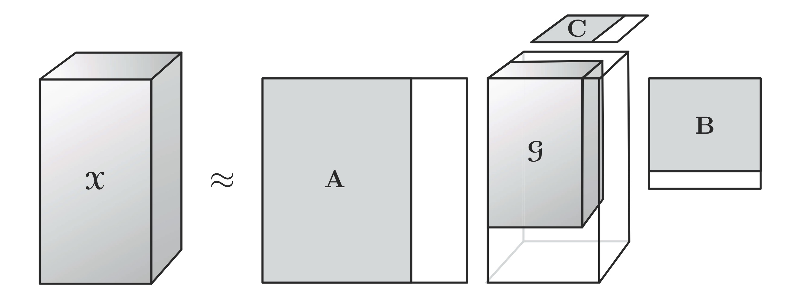
The Tucker decomposition is a form of higher-order PCA, and it decomposes a tensor into a core tensor multiplied (or transformed) by a matrix along each mode. For a third-order tensor \(\mathbfcal{X} \in \mathbb{R}^{I \times J \times K}\), \[\mathbfcal{X} \approx \mathbfcal{G} \times_1 \mathbf{A} \times_2 \mathbf{B} \times_3 \mathbf{C}=\sum_{p=1}^P \sum_{q=1}^Q \sum_{r=1}^R g_{pqr}\mathbf{a}_p \circ \mathbf{b}_q \circ \mathbf{c}_r=[\![ \mathbfcal{G}; \mathbf{A}, \mathbf{B}, \mathbf{C} ]\!]\] where \(\mathbf{A} \in \mathbb{R}^{I \times P}\), \(\mathbf{B} \in \mathbb{R}^{J \times Q}\) and \(\mathbf{C} \in \mathbb{R}^{K \times R}\) are the factor matrices (which are usually orthogonal), and can be thought of as the principal components in each mode. The tensor \(\mathbfcal{G} \in \mathbb{R}^{P \times Q \times R}\) is called the core tensor and its entries show the the level of interaction between the different components.
Elementwise, for \(i=1, \ldots, I\), \(j=1, \ldots, J\) and \(k=1, \ldots, K\), \[x_{ijk} \approx \sum_{p=1}^P \sum_{q=1}^Q \sum_{r=1}^R g_{pqr}a_{ip}b_{jq}c_{kr}\] where \(P\), \(Q\) and \(R\) are the number of components (i.e., columns) in the factor matrices \(\mathbf{A}\), \(\mathbf{B}\) and \(\mathbf{C}\), respectively. If \(P\), \(Q\) and \(R\) are smaller than \(I\), \(J\) and \(K\), the core tensor \(\mathbfcal{G}\) can be thought of as a compressed version of \(\mathbfcal{X}\).
CP and be viewed as a special case of Tucker where the core tensor is superdiagonal and \(P=Q=R\).
The Tucker decomposition in matricized form (one per mode): \[\begin{aligned} \mathbf{X}_{(1)} &\approx \mathbf{A}\mathbf{G}_{(1)}(\mathbf{C} \otimes \mathbf{B})^\top, \\ \mathbf{X}_{(2)} &\approx \mathbf{B}\mathbf{G}_{(2)}(\mathbf{C} \otimes \mathbf{A})^\top, \\ \mathbf{X}_{(3)} & \approx \mathbf{C}\mathbf{G}_{(3)}(\mathbf{B} \otimes \mathbf{A})^\top. \end{aligned}\]
In general, the Tucker decomposition is \[\mathbfcal{X} \approx [\![ \mathbfcal{G}; \mathbf{A}^{(1)}, \ldots, \mathbf{A}^{(N)} ]\!]=\mathbf{G} \times_1 \mathbf{A}^{(1)} \times_2 \cdots \times_N \mathbf{A}^{(N)}\] or elementwise, for \(i_n=1, \ldots, I_n\), \(n=1, \ldots, N\), \[x_{i_1, \ldots, i_N} \approx \sum_{r_1=1}^{R_1} \cdots \sum_{r_N=1}^{R_N} g_{r_1, \ldots, r_N} a_{i_1, r_1}^{(1)} \cdots a_{i_N, r_N}^{(N)}.\] The matricized version is \[\mathbf{X}_{(n)} \approx \mathbf{A}^{(n)}\mathbf{G}_{(n)}(\mathbf{A}^{(N)} \otimes \cdots \otimes \mathbf{A}^{(n+1)} \otimes \mathbf{A}^{(n-1)} \otimes \cdots \otimes \mathbf{A}^{(1)})^\top.\]
此外,还有两个Tucker分解的变形是值得注意的。
第一个是Tucker2分解,这个方法只使用两个矩阵来分解,第三个矩阵为单位矩阵,比如说:\[\mathbfcal{X}=\mathbfcal{G} \times_1 \mathbf{A} \times_2 \mathbf{B}=[\![\mathbfcal{G}; \mathbf{A}, \mathbf{B}, \mathbf{I}]\!].\] Tucker2分解与Tucker分解的区别在于,\(\mathbfcal{G} \in \mathbb{R}^{P \times Q \times K}\)和\(\mathbf{C}=\mathbf{I}\).
类似的,Tucker1分解只利用某一个矩阵来分解,并将剩余矩阵设为单位矩阵,比如说:\[\mathbfcal{X}=\mathbfcal{G} \times_1 \mathbf{A}=[\![\mathbfcal{G}; \mathbf{A}, \mathbf{I}, \mathbf{I}]\!].\] 这等价于一个标准的二维主成分分析,因为\(\mathbf{X}_{(1)}=\mathbf{A}\mathbf{G}_{(1)}\).
3.2. \(n\)-Rank
Let \(\mathbfcal{X}\) be an \(N\)th-order tensor of size \(I_1 \times \cdots \times I_N\). The \(n\)-rank of \(\mathbfcal{X}\), denoted \(\text{rank}_n(\mathbfcal{X})\), is the column rank of \(\mathbf{X}_{(n)}\), i.e., the \(n\)-rank is the dimension of the vector space spanned by the mode-\(n\) fibers. If we let \(R_n=\text{rank}_n(\mathbfcal{X})\) for \(n=1, \ldots, N\), then we can say that \(\mathbfcal{X}\) is a rank-\((R_1, \ldots, R_N)\) tensor. Trivially, \(R_n \leq I_n\) for all \(n=1, \ldots, N\).
For a given tensor \(\mathbfcal{X}\), we can easily find an exact Tucker decomposition of rank \((R_1, \ldots, R_N)\). If, however, we compute a Tucker decomposition of rank \((R_1, \ldots, R_N)\) where \(R_n<\text{rank}_n(\mathbfcal{X})\) for one or more \(n\), then it will be necessarily inexact and more difficult to compute. For instance, a truncated Tucker decomposition does not exactly reproduce \(\mathbfcal{X}\):
3.3. Tucker Decomposition Computation
We focus on the higher-order orthogonal iteration (HOOI) algorithm. Let \(\mathbfcal{X} \in \mathbb{R}^{I_1 \times \cdots I_N}\), the optimization problem we want to solve is \[\min_{\mathbfcal{G}, \mathbf{A}^{(1)}, \ldots, \mathbf{A}^{(N)}} \|\mathbfcal{X} - [\![ \mathbfcal{G}; \mathbf{A}^{(1)}, \ldots, \mathbf{A}^{(N)} ]\!]\|\] s.t. \(\mathbfcal{G} \in \mathbb{R}^{R_1 \times \cdots \times R_N}\), \(\mathbf{A}^{(n)} \in \mathbb{R}^{I_n \times R_n}\), and columnwise orthogonal for \(n=1, \ldots, N\). By rewriting the objective function in vectorized form as \[\| \text{vec}(\mathbfcal{X}) - (\mathbf{A}^{(N)} \otimes \cdots \otimes \mathbf{A}^{(1)}) \text{vec}(\mathbfcal{G}) \|\] it is obvious that core tensor \(\mathbfcal{G}\) must satisfy \(\mathbfcal{G}=\mathbfcal{X} \times_1 (\mathbf{A}^{(1)})^\top \times_2 \cdots \times_N (\mathbf{A}^{(N)})^\top\). Rewrite the objective function, we have \[\begin{aligned} \|\mathbfcal{X} - [\![\mathbfcal{G}; \mathbf{A}^{(1)}, \ldots, \mathbf{A}^{(N)}]\!] \|^2&=\|\mathbfcal{X}\|^2 - 2 \langle \mathbfcal{X}, [\![\mathbfcal{G}; \mathbf{A}^{(1)}, \ldots, \mathbf{A}^{(N)}]\!] \rangle + \| [\![\mathbfcal{G}; \mathbf{A}^{(1)}, \ldots, \mathbf{A}^{(N)}]\!] \|^2 \\&=\|\mathbfcal{X}\|^2 - 2 \langle \mathbfcal{X} \times_1 (\mathbf{A}^{(1)})^\top \times_2 \cdots \times_N (\mathbf{A}^{(N)})^\top, \mathbfcal{G} \rangle + \|\mathbfcal{G}\|^2 \\&=\|\mathbfcal{X}\|^2 - 2 \langle \mathbfcal{G}, \mathbfcal{G} \rangle + \|\mathbfcal{G}\|^2 \\&=\|\mathbfcal{X}\|^2-\|\mathbfcal{G}\|^2 \\&=\|\mathbfcal{X}\|^2-\|\mathbfcal{X} \times_1 (\mathbf{A}^{(1)})^\top \times_2 \cdots \times_N (\mathbf{A}^{(N)})^\top\|^2. \end{aligned}\]
We can use an ALS approach to solve. Since \(\|\mathbfcal{X}\|^2\) is constant, it is equivalent to solve \[\max_{\mathbf{A}^{(n)}} \|\mathbfcal{X} \times_1 (\mathbf{A}^{(1)})^\top \times_2 \cdots \times_N (\mathbf{A}^{(N)})^\top\|\] s.t. \(\mathbf{A}^{(n)} \in \mathbb{R}^{I_n \times R_n}\) and columnwise orthogonal. In matrix form: \[\|(\mathbf{A}^{(n)})^\top \mathbf{X}_{(n)} (\mathbf{A}^{(N)} \otimes \cdots \otimes \mathbf{A}^{(n+1)} \otimes \mathbf{A}^{(n-1)} \otimes \cdots \otimes \mathbf{A}^{(1)})\|.\] The solution can be determined using the SVD: simply set \(\mathbf{A}^{(n)}\) to be the \(R_n\) leading left singular vectors of \(\mathbf{W}=\mathbf{X}_{(n)} (\mathbf{A}^{(N)} \otimes \cdots \otimes \mathbf{A}^{(n+1)} \otimes \mathbf{A}^{(n-1)} \otimes \cdots \otimes \mathbf{A}^{(1)})\), and the method will converge to a solution where the objective function ceases to decrease, but it is not guaranteed to converge to the global optimum or even a stationary point.
The ALS algorithm to compute a rank-\((R_1, \ldots, R_N)\) Tucker decomposition for an \(N\)th-order tensor \(\mathbfcal{X}\) of size \(I_1 \times \cdots I_N\), a.k.a. HOOI, is:
| Algorithm 2 HOOI Algorithm |
|
procedure \(\texttt{HOOI}(\mathbfcal{X}, R_1, \ldots, R_N)\) initialize \(\mathbf{A}^{(n)} \in \mathbb{R}^{I_n \times R}\) for \(n=1, \ldots, N\) using \(\texttt{HOSVD}\); repeat for \(n=1, \ldots, N\) do \(\mathbfcal{Y} \leftarrow \mathbfcal{X} \times_1 (\mathbf{A}^{(1)})^\top \times_2 \cdots \times_{n-1} (\mathbf{A}^{(n-1)})^\top \times_{n+1} (\mathbf{A}^{(n+1)})^\top \times_{n+2} \cdots \times_N (\mathbf{A}^{(N)})^\top\); \(\mathbf{A}^{(n)} \leftarrow R_n\) leading left singular vectors of \(\mathbf{Y}_{(n)}\); end for until fit ceases to improve or maximum iterations exhausted; \(\mathbfcal{G} \leftarrow \mathbfcal{X} \times_1 (\mathbf{A}^{(1)})^\top \times_2 \cdots \times_N (\mathbf{A}^{(N)})^\top\); return \(\mathbfcal{G}, \mathbf{A}^{(1)}, \ldots, \mathbf{A}^{(N)}\); end procedure |
Higher-order SVD (HOSVD) is:
| Algorithm 3 HOSVD Algorithm |
|
procedure \(\texttt{HOSVD}(\mathbfcal{X}, R_1, \ldots, R_N)\) for \(n=1, \ldots, N\) do \(\mathbf{A}^{(n)} \leftarrow R_n\) leading left singular vectors of \(\mathbf{X}_{(n)}\); end for \(\mathbfcal{G} \leftarrow \mathbfcal{X} \times_1 (\mathbf{A}^{(1)})^\top \times_2 \cdots \times_N (\mathbf{A}^{(N)})^\top\); return \(\mathbfcal{G}, \mathbf{A}^{(1)}, \ldots, \mathbf{A}^{(N)}\); end procedure |
3.4. Lack of Uniqueness
Tucker decomposition is not unique. For example, consider \(\mathbfcal{X} \approx [\![\mathbfcal{G}; \mathbf{A}, \mathbf{B}, \mathbf{C}]\!]\). Let \(\mathbf{U} \in \mathbb{R}^{P \times P}\), \(\mathbf{V} \in \mathbb{R}^{Q \times Q}\) and \(\mathbf{W} \in \mathbb{R}^{R \times R}\) be nonsingular matrices, then \[[\![\mathbfcal{G}; \mathbf{A}, \mathbf{B}, \mathbf{C}]\!]=[\![\mathbfcal{G} \times_1 \mathbf{U} \times_2 \mathbf{V} \times_3 \mathbf{W}; \mathbf{AU}^{-1}, \mathbf{BV}^{-1}, \mathbf{CW}^{-1}]\!],\] i.e., we can modify the core \(\mathbfcal{G}\) without affecting the fit so long as we apply the inverse modification to the factor matrices.