1. Causal Inference
Definition 1.1 Let \(\mathcal{G}\) be a DAG, and \(p\) be a distribution Markov w.r.t. \(\mathcal{G}\). \((\mathcal{G}, p)\) is causal for \(X_V\), if \[p(x_{V-A} \mid \text{do}(x_A))=\prod_{i \in V-A} p(x_i \mid x_{\text{pa}(i)})\] for all \(A \subseteq V\) and \(x_V \in \mathcal{X}_V\).
Example 1.1 Suppose \(p\) is causal w.r.t. \(\mathcal{G}\), then \(p(y, z \mid \text{do}(x))=p(z)p(y \mid x, z)\).
            graph LR
            Z((Z)) --> X((X)) & Y((Y))
X --> Y
\(p(y, z \mid \text{do}(x))=p(z)p(y \mid x, z) \neq p(y, z \mid x)\), where \(p(y, z \mid x)=p(z \mid x)p(y \mid x, z)\).
However, we still have \[p(y \mid \text{do}(x))=\sum_z p(y, z \mid \text{do}(x))=\sum_z p(z)p(y \mid x, z)\] or \[p(z \mid \text{do}(x))=\sum_y p(y, z \mid \text{do}(x))=p(z)\sum_y p(y \mid x, z)=p(z).\]
2. Causal DAG
Lemma 2.1 (Adjustment Formula) Let \(\mathcal{G}\) be a causal DAG, then \[p(y \mid \text{do}(z))=\sum_{x_{\text{pa}(z)}} p(x_{\text{pa}(z)}) p(y \mid z, x_{\text{pa}(z)}).\]
Proof. Let \(X_V=(Y, Z, X_{\text{pa}(z)}, X_W)\) where \(X_W\) contains any other variables. Then by definition \[\begin{aligned} p(y, x_{\text{pa}(z)}, x_W \mid \text{do}(z))&=\prod_{i \in W} p(x_i \mid x_{\text{pa}(i)})p(y \mid x_{\text{pa}(y)}) p(x_{\text{pa}(z)} \mid x_{\text{pa}(\text{pa}(z))}) \\&=\frac{p(y, x_{\text{pa}(z)}, x_W, z)}{p(z \mid x_{\text{pa}(z)})} \\&=\frac{p(z \mid x_{\text{pa}(z)})p(x_{\text{pa}(z)})p(y, x_W \mid z, x_{\text{pa}(z)})}{p(z \mid x_{\text{pa}(z)})} \\&=p(x_{\text{pa}(z)})p(y, x_W \mid z, x_{\text{pa}(z)}). \end{aligned}\]
Hence, \[\begin{aligned} p(y \mid \text{do}(z))&=\sum_{x_{\text{pa}(z)}, x_W} p(y, x_{\text{pa}(z)}, x_W \mid \text{do}(z)) \\&=\sum_{x_{\text{pa}(z)}} p(x_{\text{pa}(z)})\sum_{x_W}p(y, x_W \mid z, x_{\text{pa}(z)}) \\&=\sum_{x_{\text{pa}(z)}} p(x_{\text{pa}(z)})p(y \mid z, x_{\text{pa}(z)}). \end{aligned}\]\(\square\)
Example 2.1
            graph LR
            Z((Z)) --> W((W))
T((T)) --> X((X)) --> Y((Y))
Z --> X
W --> Y
According to adjustment formula, \(\displaystyle p(y \mid \text{do}(x))=\sum_{t, z}p(t, z)p(y \mid x, t, z)\). Since \(T \perp\!\!\!\!\perp Y \mid X, Z\), then \[p(y \mid \text{do}(x))=\sum_{t, z}p(t, z)p(y \mid x, z)=\sum_z p(z)p(y \mid x, z).\]
Besides, we have \[\begin{aligned} p(y \mid \text{do}(x))&=\sum_z p(z)p(y \mid x, z) \\&=\sum_{z, w} p(z)p(y, w \mid x, z) \\&=\sum_{z, w} p(z)p(w \mid x, z)p(y \mid w, x, z) \\&=\sum_{z, w} p(z)p(w \mid z)p(y \mid w, x) \\&=\sum_{w} p(w)p(y \mid w, x) \end{aligned}\]
The example illustrates that there are often multiple equivalent ways of obtaining the same causal quantity.
3. d-Separation
Definition 3.1 Let \(\mathcal{G}\) be a DAG, and \(\pi\) be a path in \(\mathcal{G}\). We say that an internal vertex (i.e., not the first and the last vertex on \(\pi\)) \(v\) is a collider if both adjacent edges point to \(v\): \(\to v \leftarrow\). Otherwise, \(v\) is a non-collider.
Definition 3.2 Let \(\pi\) be a path from \(a\) to \(b\). We say that \(\pi\) is open conditional on \(C \subseteq V-\{a, b\}\) if:
every collider must be in \(\text{an}(C)\);
no non-collider can be in \(C\).
Otherwise, \(\pi\) is blocked or closed given \(C\).
Example 3.1
            graph LR
            Z((Z)) --> W((W))
T((T)) --> X((X)) --> Y((Y))
Z --> X
W --> Y
We have \[\begin{aligned} \pi_1&: T \to X \to Y \quad \text{(Direct causal path)}\\ \pi_2&: T \to X \leftarrow Z \to W \to Y \quad \text{(Backdoor path)} \end{aligned}\]
Given \(\varnothing\), \(\pi_1\) is open since \(X\) is a non-collider not in \(\varnothing\); \(\pi_2\) is blocked since \(X\) is a collider not in \(\text{an}(\varnothing)\).
Given \(\{X\}\), \(\pi_1\) is blocked since \(X\) is a non-collider in \(\{X\}\); \(\pi_2\) is open since \(X\) is a collider in \(\text{an}(\{X\})\).
Given \(\{X, Z\}\), \(\pi_1\) and \(\pi_2\) are blocked.
Definition 3.3 Let \(A, B, C\) be disjoint subsets of \(V\) in a DAG \(\mathcal{G}\), where \(C\) may be empty. We say \(A\) and \(B\) are d-separated given \(C\), if all paths from any \(a \in A\) to any \(b \in B\) are blocked by \(C\), denoted \(A \perp_d B \mid C\).
Theorem 3.1 Let \(\mathcal{G}\) be a DAG with disjoint subsets \(A\), \(B\) and \(C\). Then \(A \perp_s B \mid C\ [(\mathcal{G}_{\text{an}(A \cup B \cup C)})^m]\) iff \(A\) is d-separated from \(B\) by \(C\) in \(\mathcal{G}\).
4. Adjustment Set
Definition 4.1 \(C\) is an adjustment set for \((t, y)\) if \[p(y \mid \text{do}(t))=\sum_{x_C} p(x_C)p(y \mid t, x_C).\]
\(C=\text{pa}(t)\) is an adjustment set.
Definition 4.2 Given a causal effect \(T \to Y\), we define the causal nodes \(\text{cn}(T \to Y)\) to be nodes on a causal path from \(T\) to \(Y\), except for \(T\), i.e., \[\text{cn}(T \to Y)=\text{an}(Y) \cap \text{de}(T)-\{T\}.\] We define the forbidden nodes for \(T \to Y\) as consisting of \(T\) or any descendants of causal nodes, i.e., \[\text{forb}(T \to Y)=\text{de}(\text{cn}(T \to Y)) \cup \{T\}.\]
Example 4.1
            graph LR
            Z((Z)) --> W((W))
Z --> X((X))
W --> Y((Y))
T((T)) --> X --> Y --> S((S))
T --> Y
X --> R((R))
By definition \(\text{cn}(T \to Y)=\{X, Y\}\) and \(\text{forb}(T \to Y)=\{R, S, T, X, Y\}\).
Definition 4.3 Given a causal effect \(T \to Y\), we say that \(C \subseteq V-\{T, Y\}\) is a valid adjustment set if:
\(C \cap \text{forb}(T \to Y)=\varnothing\);
\(C\) must block all non-causal path from \(T\) to \(Y\).
We can divide a valid adjustment set \(C\) into two components: \[B=C \cap \text{nd}(T) \quad \text{and} \quad D=C-B=C \cap \text{de}(T).\] We call \(B\) the backdoor adjustment set.
Theorem 4.1 If \(C\) is a valid adjustment set for \((T, Y)\), then so is \(B=C \cap \text{nd}(T)\).
Proof. If \(C \cap \text{forb}(T \to Y)=\varnothing\), then \(B \cap \text{forb}(T \to Y)=\varnothing\) since \(B \subseteq C\).
Consider path from \(T\) to \(Y\). Any path beginning with an edge \(T \to \cdots\) is either causal, or will meet a collider.
Since causal path is open given \(C\), then all non-colliders are outside \(C\) and thus are outside \(B \subseteq C\), i.e., causal path is open given \(B\).
If path meeting a collider is blocked by \(C\), then the collider is not in \(\text{an}(C)\), and thus is not in \(\text{an}(B) \subseteq \text{an}(C)\), i.e., the path meeting a collider is blocked by \(B\).
Any path beginning with an edge \(T \leftarrow \cdots\) is blocked by \(C\).
If the path is blocked at a collider, then the collider is not in \(\text{an}(C)\), and thus is not in \(\text{an}(B) \subseteq \text{an}(C)\) i.e., the path is blocked by \(B\).
If the path is blocked at a non-collider that is not in \(\text{de}(T)\), then the non-collider is in \(B\), i.e., the path is blocked by \(B\).
If the path \(\pi_1\) is blocked at a non-collider that is in \(\text{de}(T)\), then the non-collider is in \(D\) and \(\pi_1\) is blocked by \(D\). Consider the path \(\pi_2\) from \(T\) to \(Y\) with \(T \to D \to \cdots\), then there must be a collider on \(\pi_2\), and thus \(\pi_1\) is blocked by \(B\).
\(\square\)
It \(C\) is a valid adjustment set for \((T, Y)\), then any superset of \(B\) that removes a set closed under taking descendants (any set \(B \cup A\) for \(A \subseteq D\) with \(\text{an}(A) \cap D=A \cap D=A\)) is a valid adjustment set for \((T, Y)\).
Theorem 4.2 For any \(d \in C-B\), either \(d \perp_d y \mid (C-\text{de}(d)) \cup \{t\}\) or \(d \perp_d t \mid C-\text{de}(d)\), where \(C\) is a valid adjustment set for \((t, y)\) and \(B=C \cap \text{nd}(t)\).
Proof. Assume for a contradiction that both statements fail. Consider \(A=\text{an}(\{d, y, t\} \cup (C-\text{de}(d)))\). In \((\mathcal{G}_A)^m\), undirected path from \(y\) to \(d\) does not intersect \((C-\text{de}(d)) \cup \{t\}\), and undirected path from \(t\) to \(d\) does not intersect \(C-\text{de}(d)\). We can concatenate these two paths to obtain an open path \(\pi\) from \(t\) to \(y\) given \(C-\text{de}(d)\), which is a contradiction.\(\square\)
Lemma 4.3 If \(C\) is a valid adjustment set and \(B=C \cap \text{nd}(t)\), then \[\sum_{x_C} p(x_C)p(y \mid t, x_C)=\sum_{x_B} p(x_B)p(y \mid t, x_B).\]
Proof. Take \(d \in C-B\) s.t. \(\text{de}(d) \cap C=\{d\}\). We know that either \(d \perp_d y \mid (C-\{d\}) \cup \{t\}\), in which case we have \[\begin{aligned} \sum_{x_C} p(x_C)p(y \mid t, x_C)&=\sum_{x_{C-\{d\}}, x_d} p(x_{C-\{d\}}, x_d)p(y \mid t, x_{C-\{d\}}, x_d) \\&=\sum_{x_{C-\{d\}}, x_d} p(x_{C-\{d\}}, x_d)p(y \mid t, x_{C-\{d\}}) \\&=\sum_{x_{C-\{d\}}} p(x_{C-\{d\}})p(y \mid t, x_{C-\{d\}}), \end{aligned}\]
or \(d \perp_d t \mid C-\{d\}\), in which case we have \[\begin{aligned} \sum_{x_C} p(x_C)p(y \mid t, x_C)&=\sum_{x_C} p(x_{C-\{d\}})p(x_d \mid x_{C-\{d\}})p(y \mid t, x_C) \\&=\sum_{x_{C-\{d\}}} p(x_{C-\{d\}}) \sum_{x_d} p(x_d \mid x_{C-\{d\}}, t)p(y \mid t, x_C) \\&=\sum_{x_{C-\{d\}}} p(x_{C-\{d\}}) \sum_{x_d} p(x_d, y \mid x_{C-\{d\}}, t) \\&=\sum_{x_{C-\{d\}}} p(x_{C-\{d\}})p(y \mid t, x_{C-\{d\}}). \end{aligned}\]
By iteratively removing such \(d\), the result holds.\(\square\)
Theorem 4.3 Let \(C\) be a valid adjustment set for \(T \to Y\), then \[p(y \mid \text{do}(t))=\sum_{x_C} p(x_C)p(y \mid t, x_C).\]
Proof. By lemma 4.2, it is sufficient to prove with assumption that \(C\) contains no descendants of \(t\). Since \(C \cap \text{de}(t) = \varnothing\), then \(t \perp_d C \mid \text{pa}(t)\) by local Markov property.
Suppose there is an open path \(\pi\) from some \(s \in \text{pa}(t)\) to \(y\) given \(C \cup \{t\}\). If \(\pi\) passes through \(t\), then \(t\) is a collider on the path, and we can shorten it to give an open path from \(t\) to \(y\) that begins \(t \leftarrow\), and thus the path from \(t\) to \(y\) is open given \(C\), which is a contradiction. If \(\pi\) is open given \(C\), then the path from \(t\) to \(y\) is open given \(C\), which is a contradiction. If \(\pi\) is not open given \(C\), then there exits a collider \(r \in \text{an}(t)-\text{an}(C)\), and there is a directed path from \(r\) to \(t\) that does not contain any element of \(C\). We concatenate the path from \(t\) to \(y\) and the path is open given \(C\). Hence, we will always obtain an open path from \(t\) to \(y\) given \(C\), which is a contradiction. Hence, \(y \perp_d \text{pa}(t) \mid C \cup \{t\}\).
Then \[\begin{aligned} p(y \mid \text{do}(t))&=\sum_{x_{\text{pa}(t)}} p(x_{\text{pa}(t)})p(y \mid t, x_{\text{pa}(t)}) \\&=\sum_{x_{\text{pa}(t)}} p(x_{\text{pa}(t)}) \sum_{x_C} p(y, x_C \mid t, x_{\text{pa}(t)}) \\&=\sum_{x_{\text{pa}(t)}} p(x_{\text{pa}(t)}) \sum_{x_C} p(y \mid t, x_{\text{pa}(t)}, x_C)p(x_C \mid t, x_{\text{pa}(t)}) \\&=\sum_{x_{\text{pa}(t)}} p(x_{\text{pa}(t)}) \sum_{x_C} p(y \mid t, x_C)p(x_C \mid x_{\text{pa}(t)}) \\&=\sum_{x_C} p(y \mid t, x_C)\sum_{x_{\text{pa}(t)}} p(x_{\text{pa}(t)})p(x_C \mid x_{\text{pa}(t)}) \\&=\sum_{x_C} p(y \mid t, x_C)\sum_{x_{\text{pa}(t)}} p(x_{\text{pa}(t)}, x_C) \\&=\sum_{x_C} p(y \mid t, x_C)p(x_C). \end{aligned}\]\(\square\)
5. Gaussian Causal Model
The adjustment formula is a way of estimating causal effect using observational distributions: \[\mathbb{E}[Y \mid \text{do}(z)]=\sum_{x_C}p(x_C)\mathbb{E}[Y \mid z, x_C].\]
For multivariate Gaussian, \(\displaystyle \mathbb{E}[Y \mid z, x_C]=\beta_0+\beta_zz+\sum_{c \in C} \alpha_cx_c\), and thus \[\begin{aligned} \mathbb{E}[Y \mid \text{do}(z)]&=\int_{\mathcal{X}_C} p(x_C)\left(\beta_0+\beta_zz+\sum_{c \in C} \alpha_cx_c\right)\text{d}x_C \\&=\beta_0+\beta_zz+\sum_{c \in C} \alpha_c\mathbb{E}[X_c]. \end{aligned}\]
The causal effect for \(Z\) on \(Y\) is \(\beta_z\).
6. Structural Equation Model
A structural equation model is a multivariate Gaussian causal model.
Recall that \(p\) is multivariate Gaussian and Markov w.r.t. a DAG \(\mathcal{G}\) iff \[X_v=\sum_{p \in \text{pa}(v)} \beta_{vp}X_p+\varepsilon_v\] where \(\varepsilon_v \sim \mathcal{N}(0, \sigma_v^2)\) and \(\varepsilon_v\)'s are independent.
In matrix form, \(X=BX+\varepsilon\) and \(X=(I-B)^{-1}\varepsilon\), where \(B\) is lower triangular, \(\varepsilon \sim \mathcal{N}_p(0, D)\), and \(D\) is diagonal. We obtain \[\Sigma=\text{Var}[X]=(I-B)^{-1}\text{Var}[\varepsilon](I-B)^{-\top}=(I-B)^{-1}D(I-B)^{-\top}.\]
We know \[(B^2)_{ij}=\sum_{k=1}^p \beta_{ik}\beta_{kj}\] and \(\beta_{ik}\beta_{kj} \neq 0\) only if \(j \to j \to i\) is a directed path in \(\mathcal{G}\). Similarly, \[(B^3)_{ij}=\sum_{k=1}^p\sum_{l=1}^p \beta_{ik}\beta_{kl}\beta_{lj}\] and \(\beta_{ik}\beta_{kl}\beta_{lj} \neq 0\) only if \(j \to l \to k \to i\) is a directed path in \(\mathcal{G}\). Since the max path length in \(\mathcal{G}\) is \(p-1\), then \(B^p=0\), i.e., \(B\) is nilpotent.
Since \(B\) is nilpotent, then \((I-B)(I+B+B^2+\cdots+B^{p-1})=I\), i.e., \[(I-B)^{-1}=I+B+B^2+\cdots+B^{p-1}.\]
Example 6.1 Consider a DAG
            graph LR
            X((X)) --> |β| Z((Z))
X --> |α| Y((Y))
Y --> |γ| Z
with \(X=\varepsilon_x\), \(Y=\alpha X+\varepsilon_y\), and \(Z=\beta X+\gamma Y+\varepsilon_z\) for \((\varepsilon_x, \varepsilon_y, \varepsilon_z)^\top \sim \mathcal{N}_3(0, I)\). The matrix form is \[\begin{bmatrix} X \\ Y \\ Z \end{bmatrix}=\begin{bmatrix} 0 & 0 & 0 \\ \alpha & 0 & 0 \\ \beta & \gamma & 0 \end{bmatrix}\begin{bmatrix} X \\ Y \\ Z \end{bmatrix}+\begin{bmatrix} \varepsilon_x \\ \varepsilon_y \\ \varepsilon_z \end{bmatrix}\] which is equivalent to \[\begin{bmatrix} 1 & 0 & 0 \\ -\alpha & 1 & 0 \\ -\beta & -\gamma & 1 \end{bmatrix}\begin{bmatrix} X \\ Y \\ Z \end{bmatrix}=\begin{bmatrix} \varepsilon_x \\ \varepsilon_y \\ \varepsilon_z \end{bmatrix}.\] Therefore, \[(I-B)^{-1}=\begin{bmatrix} 1 & 0 & 0 \\ -\alpha & 1 & 0 \\ -\beta & -\gamma & 1 \end{bmatrix}^{-1}=\begin{bmatrix} 1 & 0 & 0 \\ \alpha & 1 & 0 \\ \beta+\alpha\gamma & \gamma & 1 \end{bmatrix}\] and \[\Sigma=(I-B)^{-1}D(I-B)^{-\top}=\begin{bmatrix} 1 & \alpha & \beta+\alpha\gamma \\ \alpha & 1+\alpha^2 & \alpha\beta+\alpha^2\gamma+\gamma \\ \beta+\alpha\gamma & \alpha\beta+\alpha^2\gamma+\gamma & 1+\beta^2+\gamma^2+2\alpha\beta\gamma+\alpha^2\gamma^2 \end{bmatrix}.\]
Definition 6.1 Let \(\mathcal{G}\) be a DAG with variables \(V\). A trek from \(i\) to \(j\) with source \(k\) is a pair \((\pi_l, \pi_r)\) or directed paths, where \(\pi_l\) is directed from \(k\) to \(i\), and \(\pi_r\) is directed from \(k\) to \(j\).
A vertex may be in both the left and right sides (\(\pi_l\) and \(\pi_r\)).
We may have \(i=k\) or \(j=k\) or both.
Example 6.2 Consider a DAG
            graph LR
            X((X)) --> Z((Z))
X --> Y((Y))
Y --> Z
The treks from \(Y\) to \(Z\) are: \(Y \to Z\), \(Y \leftarrow X \to Z\), and \(Y \leftarrow X \to Y \to Z\).
The treks from \(Z\) to \(Z\) are: \(Z\), \(Z \leftarrow X \to Z\), \(Z \leftarrow Y \to Z\), \(Z \leftarrow X \to Y \to Z\), \(Z \leftarrow Y \leftarrow X \to Z\), and \(Z \leftarrow Y \leftarrow X \to Y \to Z\).
Definition 6.2 Let \(\tau=(\pi_l, \pi_r)\) be a trek with source \(k\). The trek covariance associated with \(\tau\) is \[c(\tau)=d_{kk}\left(\prod_{(i \to j) \in \pi_l} \beta_{ji}\right)\left(\prod_{(i \to j) \in \pi_r} \beta_{ji}\right).\]
An empty product is \(1\) by convention.
Example 6.3 Consider a DAG
            graph LR
            X((X)) --> |β| Z((Z))
X --> |α| Y((Y))
Y --> |γ| Z
Trek covariances include \(c(Z)=1\), \(c(Z \leftarrow X)=\beta\), \(c(Z \leftarrow X \to Y \to Z)=\beta\alpha\gamma\), and \(c(Y \to Z)=\gamma\).
Theorem 6.1 (Trek Rule) Let \(\Sigma=(I-B)^{-1}D(I-B)^{-\top}\) be a covariance matrix that is Markov w.r.t. a DAG \(\mathcal{G}\). Then \[\sigma_{ij}=\sum_{\tau \in \mathcal{T}_{ij}} c(\tau)\] where \(\mathcal{T}_{ij}\) is the set of treks from \(i\) to \(j\).
Proof. For \(p=1\), \(\sigma_{11}=d_{11}\).
Suppose the trek rule is true for \(|V| \leq p-1\). For \(\text{Cov}(X_i, X_j)\), where \(i, j<p\), we know the trek rule holds by induction hypothesis. Since \[X_p=\sum_{i \in \text{pa}(p)} \beta_{pi}X_i+\varepsilon_p,\] then for \(j<p\), \[\begin{aligned} \text{Cov}(X_p, X_j)&=\sum_{i \in \text{pa}(p)} \beta_{pi}\text{Cov}(X_i, X_j)+\text{Cov}(X_j, \varepsilon_p) \\&=\sum_{i \in \text{pa}(p)} \beta_{pi}\sum_{\tau \in \mathcal{T}_{ij}} c(\tau)+0. \end{aligned}\] Since any trek from \(p\) to \(j\) must consist of the combination of \(p \leftarrow i\) for some parent \(i\) of \(p\), and a trek from \(i\) to \(j\), then \[\text{Cov}(X_p, X_j)=\sum_{i \in \text{pa}(p)} \beta_{pi}\sum_{\tau \in \mathcal{T}_{ij}} c(\tau)=\sum_{\tau \in \mathcal{T}_{pj}} c(\tau).\]
Besides, \[\begin{aligned} \text{Cov}(X_p, X_p)&=\sum_{i \in \text{pa}(p)} \beta_{pi}\text{Cov}(X_i, X_p)+\text{Cov}(X_p, \varepsilon_p) \\&=\sum_{i \in \text{pa}(p)} \beta_{pi} \sum_{\tau \in \mathcal{T}_{ip}} c(\tau)+\text{Var}[\varepsilon_p] \\&=\sum_{\substack{\tau \in \mathcal{T}_{pp} \\ \tau \neq \{p\}}} c(\tau)+d_{pp} \\&=\sum_{\tau \in \mathcal{T}_{pp}} c(\tau). \end{aligned}\]\(\square\)
Example 6.4 Consider a DAG
            graph LR
            3((3)) --> 2((2)) & 4((4))
1((1)) --> 2 --> 4
For example, \[\text{Cov}(X_2, X_2)=d_{22}+\beta_{23}^2d_{33}+\beta_{21}^2d_{11}\] and \[\text{Cov}(X_2, X_4)=\beta_{42}d_{22}+\beta_{23}\beta_{43}d_{33}+\beta_{23}^2\beta_{42}d_{33}+\beta_{21}^2\beta_{42}d_{11}.\]
7. Optimal Adjustment Set
The set \(O\) is optimal in that: \(\text{Var}[\widehat{\beta}_{ty \cdot O}]\) is minimal; no subset of \(O\) will give the same variance. \(\widehat{\beta}_{ty \cdot O}\) is the least squares estimator of regression coefficient that is the effect of \(T\) on \(Y\) conditional on the variables in \(O\).
Proposition 7.1 Let \(\widehat{\beta}_{Cy}=(\widehat{\beta}_{cy \cdot C'})_{c \in C}\), where \(C'=C-\{c\}\), be the least squares estimator of \(\beta_{Cy}\), where \(Y \in \mathbb{R}^n\) and \(X_C \in \mathbb{R}^{n \times q}\), then \[\sqrt{n}(\widehat{\beta}_{Cy}-\beta_{Cy}) \overset{d}{\to} \mathcal{N}_q(0, \sigma_{yy \cdot C}\Sigma_{CC}^{-1}).\]
Proof. We know \[\begin{aligned} \widehat{\beta}_{Cy}&=(X_C^\top X_C)^{-1}X_C^\top Y \\&=\left(\frac{1}{n}X_C^\top X_C\right)^{-1}\left(\frac{1}{n}X_C^\top Y\right) \\&=\left(\frac{1}{n}X_C^\top X_C\right)^{-1}\left(\frac{1}{n}X_C^\top(X_C\beta_{Cy}+\varepsilon_y)\right) \\&=\beta_{Cy}+\left(\frac{1}{n}X_C^\top X_C\right)^{-1}\left(\frac{1}{n}X_C^\top\varepsilon_y\right). \end{aligned}\]
By the law of large numbers, \(\displaystyle \frac{1}{n}X_C^\top X_C \overset{p}{\to} \Sigma_{CC}\), then \[\sqrt{n}(\widehat{\beta}_{Cy}-\beta_{Cy})=\Sigma_{CC}^{-1}\frac{1}{\sqrt{n}}X_C^\top\varepsilon_y+\mathcal{O}_p(1).\]
It is obvious that \(\mathbb{E}[\sqrt{n}(\widehat{\beta}_{Cy}-\beta_{Cy})] \overset{p}{\to} 0\) since \(\mathbb{E}[\varepsilon_y]=0\) and \(\mathbb{E}[\mathcal{O}_p(1)] \overset{p}{\to} 0\). Besides, \[\text{Var}[\sqrt{n}(\widehat{\beta}_{Cy}-\beta_{Cy})] \overset{p}{\to} \Sigma_{CC}^{-1}\Sigma_{CC}(I_n\sigma_{yy \cdot C})\Sigma_{CC}^{-\top}=\sigma_{yy \cdot C}\Sigma_{CC}^{-1}.\]\(\square\)
Proposition 7.2 Suppose \(C\) and \(D\) are valid adjustment sets for \(T \to Y\). Let \(C'=C-D\) and \(D'=D-C\). If \(Y \perp\!\!\!\!\perp X_{D'} \mid X_C, T\) and \(T \perp\!\!\!\!\perp X_{C'} \mid X_D\), then \[\frac{\sigma_{yy \cdot tC}}{\sigma_{tt \cdot C}} \leq \frac{\sigma_{yy \cdot tD}}{\sigma_{tt \cdot D}}.\]
Proof. Note that \(C \cup D=C' \cup D=C \cup D'\). Since \(Y \perp\!\!\!\!\perp X_{D'} \mid X_C, T\), then \(\sigma_{yy \cdot tC}=\sigma_{yy \cdot tCD'}=\sigma_{yy \cdot tC'D}\). If we remove elements from the conditioning set, the residual variance of \(Y\) will only increase or not change, i.e., \(\sigma_{yy \cdot tC}=\sigma_{yy \cdot tC'D} \leq \sigma_{yy \cdot tD}\). Since \(T \perp\!\!\!\!\perp X_{C'} \mid X_D\), then \(\sigma_{tt \cdot D}=\sigma_{tt \cdot C'D}=\sigma_{tt \cdot CD'} \leq \sigma_{tt \cdot C}\). Hence, \[\frac{\sigma_{yy \cdot tC}}{\sigma_{tt \cdot C}} \leq \frac{\sigma_{yy \cdot tD}}{\sigma_{tt \cdot D}}.\]\(\square\)
Definition 7.1 Given a causal graph \(\mathcal{G}\) and a distribution that is Markov w.r.t. \(\mathcal{G}\), the optimal adjustment set is \[O(T \to Y)=\text{pa}(\text{cn}(T \to Y))-(\text{cn}(T \to Y) \cup \{T\}).\]
Example 7.1 Consider the causal graph:
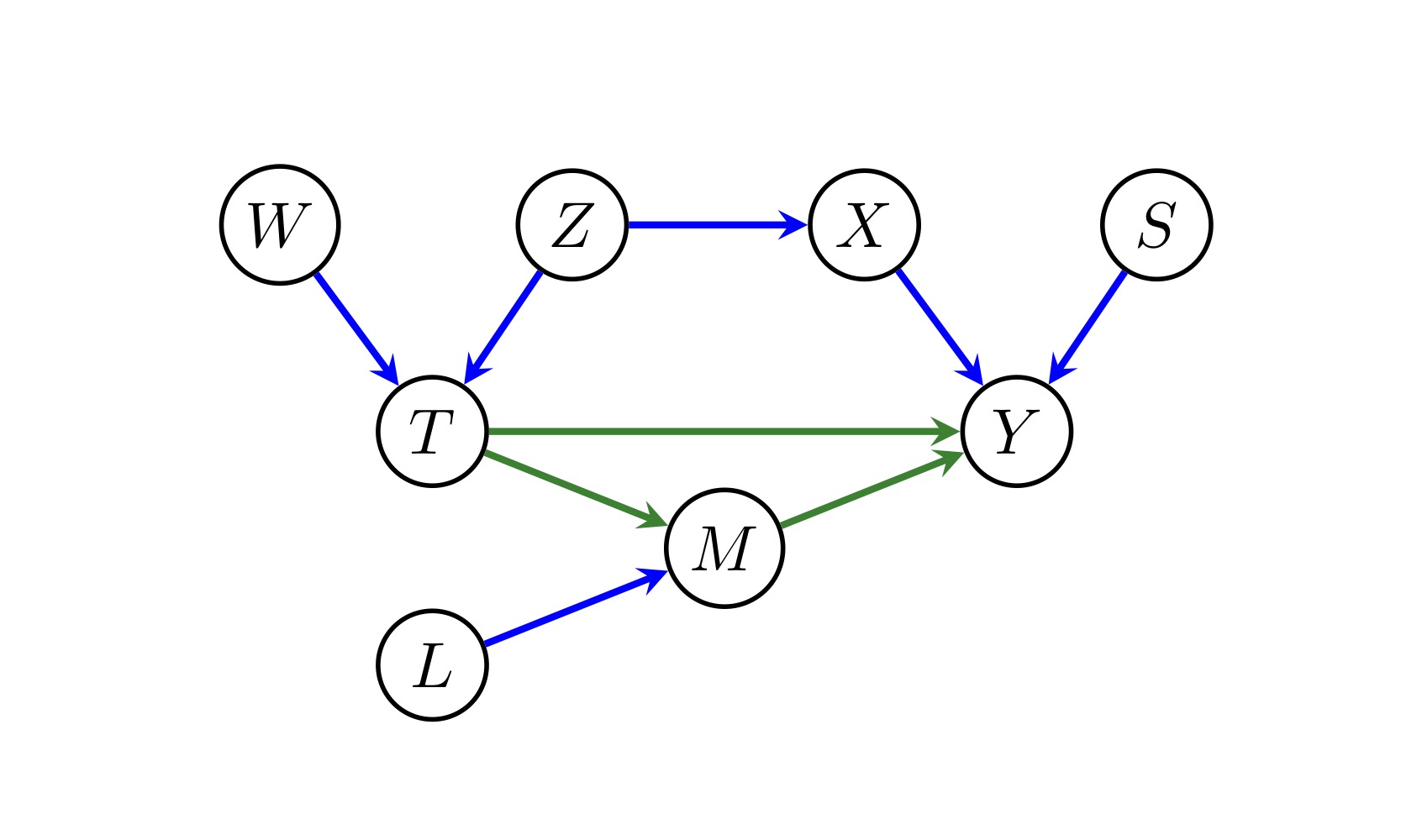
Since \(\text{cn}(T \to Y)=\text{an}(Y) \cap \text{de}(T)-\{T\}=\{M, Y\}\), then \(\text{pa}(\text{cn}(T \to Y))=\{T, L, M, X, S\}\), and thus \(O(T \to Y)=\{T, L, M, X, S\}-\{M, Y, T\}=\{X, S, L\}\). Hence, we choose to block \(X\), and adjust \(S\) and \(L\).
Theorem 7.3 Let \(\mathcal{G}\) be a causal DAG containing variables \(T\) and \(Y\). Then the set \(O(T \to Y)\) is a valid adjustment set, and the asymptotic variance of \(\widehat{\beta}_{ty \cdot O}\) is minimal over all valid adjustment sets.
Proof. \(O\) contains no descendants of \(T\), and any non-causal path from \(T\) to \(Y\) is blocked since any such path will have a conditioned non-collider as the node immediately before it meets \(\text{cn}(T \to Y)\). Hence \(O\) is a valid adjustment set.
Suppose \(Z\) is a valid adjustment set, \(O'=O-Z\), and \(Z'=Z-O\). Since \((Z \cup O) \cap \text{forb}(T \to Y)=\varnothing\), then any path (from \(Y\) to vertex in \(Z'\)) that descends at any point from a node in \(\text{cn}(T \to Y)\) are blocked. Any path (from \(Y\) to vertex in \(Z'\)) that does not descend from \(\text{cn}(T \to Y)\) must meet a parent of \(\text{cn}(T \to Y)\), i.e., either \(T\) or vertex in \(O\), which is a non-collider on the path, and thus the path is blocked. Hence, \(Y \perp_d Z' \mid O \cup \{T\}\).
If there is an open path from \(T\) to \(o \in O'\), then we can concatenate with a directed causal path to \(Y\) through \(\text{cn}(T \to Y)\), and obtain that \(Z\) is not a valid adjustment set, which is a contradiction. Hence, \(T \perp_d O' \mid Z\).
Therefore, by proposition 7.2, \(O(T \to Y)\) has minimal variance.\(\square\)